Measuring lights at night
An exploratory analysis of the NPP-VIIRS Day/Night band PSF disaggregation.
If you want the story of this analysis, start with the blog: https://daynan.com/at-the-edge/measuring-lights-at-night/
This notebook is a more detailed documentation of the experiment and results. Every number is computed from a checksummed
artifact in outputs/psf_disaggregation/; nothing is transcribed by hand.
A note on AI and science Some aspects of science are tedious work and while the limits of AI are real and important to consider, I believe leveraging it as a tool to track my specific decisions and versions and experimental trials has allowed me to document my approach more comprehensively and efficiently than I could have done otherwise. It also saved me weeks of implementation, which has an impact on choices of experiment design and execution.
You've heard of cherry-picking results...I'd call avoiding even attempting such experiments as cherry-picking the initiative. It's hard to over-state how insidious the temptation and large the opportunity cost to avoid work that can be scientifically useful but not a good headline.
But - because I could do this in less than a week, I decided it was worth the effort to run an experiment that wasn't likely to produce eye-popping results even though it absolutely gave me some interesting insight into my larger problem with science I can stand behind. And most importantly, a structure for the error. For me, this is the beauty of scientific progress. And it was fun.
So here's how I used both Code and Claude on this project and the division of labor:
Me: I designed and architected this experiment. As a data scientist, my personal focus is on defining the problem space, including the science involved, selecting and evaluating the data, experiment design and method development and choice as well as investigating the results, interpretation and writing final content. I made every design choice, although low-level decisions (such as file management strategy) I delegated to AI.
Claude: some initial literature search and as a reviewer of experiment design, results, and framing. e.g. it noticed that I was referencing results figures that were from an outdated version of my validation trial, an easy fix but would have been confusing for any reviewers.
Codex: Codex built the data pipelines (would have taken me days) and drafted the accompanying technical documentation including the initial outline of this notebook. And coding the matplotlib figures, my god that alone used to take me hours. Axes, colormaps... IFYKYK.
I stand behind the code in this repo (both mine and AI-developed) and there can be mistakes in either case. I invite review and feedback and I'm particularly interested in anyone who's worked on VIIRS PSF characterization. I find open source a powerful approach and I invite scrutiny.
Let me repeat that because it's important: I believe open data and source code is essential to ensure that using AI as a tool for science is done effectively.
0. Reporting contract
When I started out, I used fairly strict rules on what constitutes a "good image" in terms of number of observations, cloud coverage, etc. Mid-way through the experiment I realized this left gaps in coverage and, given this was exploratory, I loosened the VNP Quality Assurance (QA) contract for the final spatial reporting products. The broad-QA radiance was used for built form in both cities and for the New York S2-only spatial ablation. Due to time constraints, the Delhi S2-only spatial raster was not regenerated and remains from the first strict-QA version. Therefore worth noting up front:
- The S2-only spatial ablation uses a mixed QA contract: New York is broad-QA, while Delhi remains strict-v1. Its held-out numbers are broad-QA in both cities, because the broad held-out run covers both cities on the same frozen cohort. The two displayed S2 maps are therefore not a like-for-like cross-city comparison.
- Strict-QA results are reported as footnotes throughout section 8. In every case they reproduce the sign and the ordering of the broad result. That robustness is itself evidence and is not buried.
"""Setup: paths, palette, helpers. Run this first."""
from __future__ import annotations

import hashlib
import json
from pathlib import Path

import matplotlib as mpl
import matplotlib.pyplot as plt
import numpy as np
import pandas as pd
import rasterio
import yaml
from matplotlib.colors import LinearSegmentedColormap

REPO = Path.cwd().parent if Path.cwd().name == "notebooks" else Path.cwd()
OUT = REPO / "outputs" / "psf_disaggregation"
VAL = OUT / "validation"
RAS = OUT / "rasters" / "full_city"
CONFIG_PATH = REPO / "configs" / "psf_disaggregation.yaml"
SAVEFIG_PATH = REPO / "docs" / "figures"
SAVEFIG_PATH.mkdir(parents=True, exist_ok=True)

CITIES = ["usa_new_york", "india_delhi"]
CITY_LABEL = {"usa_new_york": "New York", "india_delhi": "Delhi"}

BROAD = RAS / "v2_broad_qa_reporting"
STRICT = RAS / "v1_resumable_tiled"
PRIMARY = "built_form_primary__no_water_prior__circular_mean_reference__broad_qa"
S2_STRICT = "s2_only_ablation__no_water_prior__circular_mean_reference"

# --- palette (validated categorical order; see dataviz reference palette) -----
BLUE, ORANGE, AQUA, YELLOW, MAGENTA, GREEN, VIOLET, RED = (
    "#2a78d6", "#eb6834", "#1baf7a", "#eda100",
    "#e87ba4", "#008300", "#4a3aa7", "#e34948",
)
INK, INK_2, MUTED = "#0b0b0b", "#52514e", "#8a8984"
GRID = "#e6e5e1"

# role assignments held fixed across every figure in this notebook
COLOR = {
    "structural": BLUE,
    "neighbors": ORANGE,
    "built_form_primary": BLUE,
    "s2_only_ablation": AQUA,
    "direct": MUTED,
    "uniform": INK_2,
    "improve": BLUE,   # diverging cool pole: error goes down
    "harm": RED,       # diverging warm pole: error goes up
}

# single-hue sequential ramp for radiance magnitude (never a rainbow)
BLUE_RAMP = LinearSegmentedColormap.from_list(
    "nocturne_blue",
    ["#fcfcfb", "#cde2fb", "#9ec5f4", "#5598e7", "#2a78d6", "#184f95", "#0d366b"],
)

mpl.rcParams.update({
    "figure.dpi": 120,
    "savefig.dpi": 120,
    "font.size": 9,
    "axes.edgecolor": GRID,
    "axes.labelcolor": INK_2,
    "axes.titlesize": 10,
    "axes.titlelocation": "left",
    "axes.titlecolor": INK,
    "axes.spines.top": False,
    "axes.spines.right": False,
    "xtick.color": INK_2,
    "ytick.color": INK_2,
    "grid.color": GRID,
    "grid.linewidth": 0.6,
    "legend.frameon": False,
})


def load_json(path: Path):
    with open(path) as fh:
        return json.load(fh)


def sha256_file(path: Path) -> str:
    h = hashlib.sha256()
    with open(path, "rb") as fh:
        for chunk in iter(lambda: fh.read(1 << 20), b""):
            h.update(chunk)
    return h.hexdigest()


def band(path: Path, index: int, window=None) -> np.ndarray:
    with rasterio.open(path) as src:
        return src.read(index, window=window, masked=False)


def band_names(path: Path) -> list[str]:
    with rasterio.open(path) as src:
        return list(src.descriptions)


CONFIG = yaml.safe_load(open(CONFIG_PATH))
print(f"repo   : {REPO}")
print(f"cities : {', '.join(CITY_LABEL.values())}")
repo   : /home/daynan/research/ntl-psf-disaggregation
cities : New York, Delhi
"""Artifact inventory. Every path this notebook reads, checked up front."""
ARTIFACTS = {
    "config": CONFIG_PATH,
    "selection_v2_broad": VAL / "gate2/primary_selection/v2_broad_qa_reporting/selection.json",
    "selection_v1_strict": VAL / "gate2/primary_selection/v1_post_gate2/selection.json",
    "evidence_v2": VAL / "gate2/closeout/v2_broad_qa_reporting/evidence_classification.json",
    "headline_v2": VAL / "gate2/closeout/v2_broad_qa_reporting/headline_metrics.csv",
    "headline_v1": VAL / "gate2/closeout/v1_bounded_method_closeout/headline_metrics.csv",
    "heldout_broad": VAL / "gate2/heldout/v3_physics_buffered_native_cell_broad_qa/summary.csv",
    "heldout_broad_gain": VAL / "gate2/heldout/v3_physics_buffered_native_cell_broad_qa/gain_summary.csv",
    "heldout_broad_retain": VAL / "gate2/heldout/v3_physics_buffered_native_cell_broad_qa/sample_retention.csv",
    "heldout_strict": VAL / "gate2/heldout/v2_physics_buffered_native_cell/summary.csv",
    "heldout_strict_gain": VAL / "gate2/heldout/v2_physics_buffered_native_cell/gain_summary.csv",
    "water_broad": VAL / "gate2/broad_reporting/v1_coverage_and_water_inland/water_inland_ratio.csv",
    "water_strict": VAL / "gate2/day4_allocated_direct_ratio/v1_existing_matched_inland_control/region_metrics.csv",
    "water_compare_strict": VAL / "gate2/day4_allocated_direct_ratio/v1_existing_matched_inland_control/water_vs_inland_comparison.csv",
    "shoreline_summary": VAL / "gate2/shoreline/v1_overture_mapped_water/summary.csv",
    "shoreline_strata": VAL / "gate2/shoreline/v1_overture_mapped_water/waterfront_infrastructure_strata.csv",
    "kernel_sensitivity": VAL / "gate2/sensitivity/v1_full_city_sensitivity/kernel_sensitivity.csv",
    "obs_conditions": VAL / "gate2/observation_conditions/v1_daily_coarse_operator/condition_summary.csv",
    "gate1_closeout": VAL / "gate1/full_city_machine_closeout.md",
    "gate0_builtform": VAL / "gate0/v3_qa_grid_halo_datatake_support/built_form_gate0_summary.csv",
    "gate0_s2": VAL / "gate0/v3_qa_grid_halo_datatake_support/s2_only_gate0_summary.csv",
    "gate0_regen": VAL / "gate0/v3_qa_grid_halo_datatake_support/gate0_figure_regeneration.json",
    "manifest_broad": BROAD / "artifact_manifest.json",
}
for city in CITIES:
    ARTIFACTS[f"primary_{city}"] = BROAD / city / PRIMARY / "products.tif"
    ARTIFACTS[f"direct_{city}"] = BROAD / city / "direct_upsample__broad_qa" / "products.tif"
    ARTIFACTS[f"uniform_{city}"] = BROAD / city / "uniform_normalized_convolution__broad_qa" / "products.tif"
    ARTIFACTS[f"trust_{city}"] = BROAD / city / PRIMARY / "trust_indicators.tif"
    ARTIFACTS[f"s2_{city}"] = STRICT / city / S2_STRICT / "products.tif"
    ARTIFACTS[f"structure_{city}"] = OUT / "rasters/day2_inputs" / city / "overture_structure_bundle.tif"

inventory = pd.DataFrame(
    [{"key": k, "exists": p.exists(),
      "size_mb": round(p.stat().st_size / 1e6, 1) if p.exists() else None}
     for k, p in ARTIFACTS.items()]
)
missing = inventory.loc[~inventory.exists, "key"].tolist()
print(f"{int(inventory.exists.sum())}/{len(inventory)} artifacts present")
if missing:
    print("MISSING:", missing)
inventory
35/35 artifacts present
| key | exists | size_mb | |
|---|---|---|---|
| 0 | config | True | 0.0 |
| 1 | selection_v2_broad | True | 0.0 |
| 2 | selection_v1_strict | True | 0.0 |
| 3 | evidence_v2 | True | 0.0 |
| 4 | headline_v2 | True | 0.0 |
| 5 | headline_v1 | True | 0.0 |
| 6 | heldout_broad | True | 0.1 |
| 7 | heldout_broad_gain | True | 0.0 |
| 8 | heldout_broad_retain | True | 0.0 |
| 9 | heldout_strict | True | 0.1 |
| 10 | heldout_strict_gain | True | 0.0 |
| 11 | water_broad | True | 0.0 |
| 12 | water_strict | True | 0.0 |
| 13 | water_compare_strict | True | 0.0 |
| 14 | shoreline_summary | True | 0.0 |
| 15 | shoreline_strata | True | 0.1 |
| 16 | kernel_sensitivity | True | 0.0 |
| 17 | obs_conditions | True | 0.0 |
| 18 | gate1_closeout | True | 0.0 |
| 19 | gate0_builtform | True | 0.0 |
| 20 | gate0_s2 | True | 0.0 |
| 21 | gate0_regen | True | 0.0 |
| 22 | manifest_broad | True | 0.0 |
| 23 | primary_usa_new_york | True | 275.4 |
| 24 | direct_usa_new_york | True | 13.8 |
| 25 | uniform_usa_new_york | True | 272.4 |
| 26 | trust_usa_new_york | True | 105.6 |
| 27 | s2_usa_new_york | True | 276.8 |
| 28 | structure_usa_new_york | True | 41.5 |
| 29 | primary_india_delhi | True | 277.6 |
| 30 | direct_india_delhi | True | 13.2 |
| 31 | uniform_india_delhi | True | 273.5 |
| 32 | trust_india_delhi | True | 127.6 |
| 33 | s2_india_delhi | True | 277.6 |
| 34 | structure_india_delhi | True | 35.6 |
1. Objective
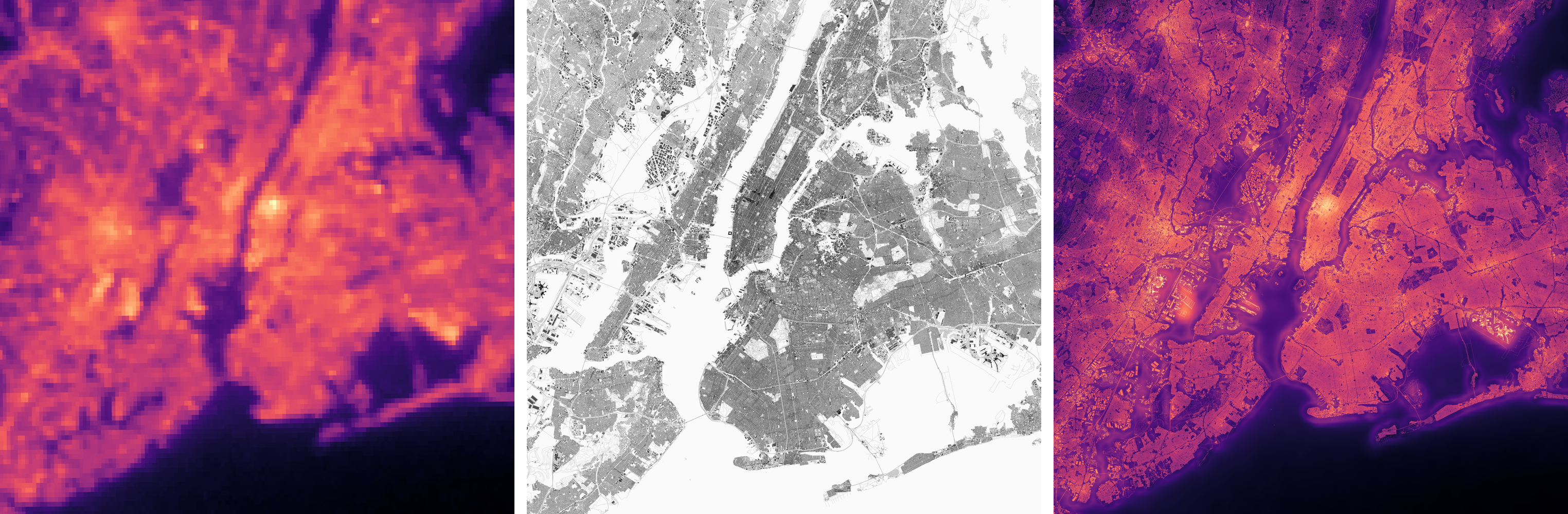
From observation to allocation. Directly upsampled VIIRS radiance (left), the structural proxy $\rho$ (center), and the structure-based 10 m allocation (right). The proxy redistributes the observed radiance; it does not replace its radiometric authority.
The question is not can we downscale nighttime lights. Dasymetric allocation and learned super-resolution are established; DeepLight and its successors produce plausible fine-grid NTL, and the literature on population-weighted dasymetric mapping goes back decades.
The question this sprint asks is narrower and, I think, more useful:
When is disaggregating a coarse observation a legitimate measurement operation, and how would you know when it isn't?
This drives the thesis of my larger overal project. Causal inference on Earth observation needs a measurement layer with an explicit error structure — otherwise every downstream estimate inherits an unknown observation term and calls it signal. Nighttime lights are the sharpest case of the problem, because the dominant sensor is spectrally blunt, view-angle dependent, and coarse relative to the built structure that produces the light. This sprint takes one specific disaggregation operator, gives it every advantage, and then tries to establish exactly what it does and does not license you to claim.
The answer, worked out below, is a bounded method result: coarse-cell prediction is validated, within-cell allocation is not, and the boundary between them is measurable rather than rhetorical.
2. The operator
The structure-based allocation, on one explicitly aligned grid:
$$ \widetilde{L}(x) \;=\; \rho(x)\,\frac{[k \otimes l](x)}{\max\big([k \otimes \rho](x),\, \varepsilon\big)} $$
where $l$ is the coarse radiance field, $\rho$ is a nonnegative structural proxy normalized to mean one, and $k$ is a declared kernel. There are no learned parameters. Nothing here is fit to anything. Therefore there is no risk of over-fitting (as well as requiring massive computational and data storage resources for training data).
Read it as a share: within each kernel neighborhood, distribute the observed radiance in proportion to $\rho$. That reading is what makes the properties below follow from algebra rather than from a training run.
Properties of the kernel
1. The proxy's scale cancels exactly. $\rho$ appears once in the numerator and once inside the convolution in the denominator, so replacing $\rho$ with $c\rho$ for any $c>0$ leaves $\widetilde{L}$ unchanged (up to the $\varepsilon$ floor). The proxy needs no units, no calibration, and no relationship to radiance in absolute terms. It only needs to encode relative within-neighborhood allocation. This is why a dimensionless mixture of building fraction and road density can be used at all.
2. The failure mode is closed-form and local. The only way the operator can misbehave numerically is a small denominator: $[k \otimes \rho](x) \to 0$. That is a computable scalar field, not an emergent property of a fit, so it can be thresholded, masked, and included as a diagnostic band that is explicitly mapped to every cell in the output layer.
3. Local normalization and not conservation. The coarse observation enters the numerator of every output neighborhood, so the observation constrains the output everywhere. But the local gain $\rho(x)/[k \otimes \rho](x)$ varies spatially, so re-aggregating the fine field does not algebraically return the coarse field. In other words, the output of this kernel will not exactly equal the radiance of the original input radiance. Again, this residiual (from input radiance to re-aggregated allocation) is included explicitly as a band in the raster image, so this is error is transparent.
Below you can see this actual residual (difference in input radiance and re-aggreagated allocation) -- it isn't trivial, but the larger ongoing work here is that this residual represents uncertainty that can be further quantified.
"""What reaggregation error actually measures on the reporting-primary product."""
rows = []
for city in CITIES:
    m = load_json(BROAD / city / PRIMARY / "metrics.json")["metrics"]
    direct = band(ARTIFACTS[f"direct_{city}"], 1)
    mean_abs = float(np.nanmean(np.abs(direct)))
    rows.append({
        "city": CITY_LABEL[city],
        "consistency_MAE": m["operator_consistency_mae"],
        "consistency_RMSE": m["operator_consistency_rmse"],
        "consistency_bias": m["operator_consistency_bias"],
        "mean_abs_source_radiance": mean_abs,
        "MAE_pct_of_mean": 100 * m["operator_consistency_mae"] / mean_abs,
    })
    del direct

consistency = pd.DataFrame(rows)
display(consistency.round(3))

print(
    "\nReaggregating the 10 m field returns the coarse observation to within "
    f"{consistency.MAE_pct_of_mean.min():.1f}-{consistency.MAE_pct_of_mean.max():.1f}% "
    "of mean absolute source radiance."
    "\nThat is a real residual, not a rounding artifact. The registered term for "
    "this operator is\n'locally normalized', and the config sets "
    "maximum_error_for_conserving_language = null, i.e. no error threshold has\n"
    "been declared that would license conserving language."
)
/tmp/ipykernel_4640/2449412562.py:92: DeprecationWarning: Setting the shape on a NumPy array has been deprecated in NumPy 2.5.
As an alternative, you can create a new view using np.reshape (with copy=False if needed).
  return src.read(index, window=window, masked=False)
| city | consistency_MAE | consistency_RMSE | consistency_bias | mean_abs_source_radiance | MAE_pct_of_mean | |
|---|---|---|---|---|---|---|
| 0 | New York | 5.342 | 9.907 | 0.559 | 43.638 | 12.242 |
| 1 | Delhi | 3.885 | 6.379 | 0.572 | 37.222 | 10.437 |
Reaggregating the 10 m field returns the coarse observation to within 10.4-12.2% of mean absolute source radiance.
That is a real residual, not a rounding artifact. The registered term for this operator is
'locally normalized', and the config sets maximum_error_for_conserving_language = null, i.e. no error threshold has
been declared that would license conserving language.
The one configuration where reaggregation is near-exact is the native-footprint kernel, which aggregates over the actual 15-arcsecond VNP cell polygons instead of a circular window. There, cell-level normalized consistency MAE is 0.10–0.16 (Gate 1 full-city closeout), roughly two orders of magnitude tighter.
That contrast is informative: the discrepancy is a property of the kernel choice, not of the algebra. A circular 500 m window is not the partition the observation actually lives on, so shares computed against it do not close.
3. The Fork et al. analogy, and its two breaks
The algebraic form comes from Fork et al. (2026), Estimating high-resolution albedo for urban applications (paper, code), where it performs a training-free convolution calibration between corresponding high- and low-resolution reflectance bands.
Two breaks are important to note here as they impact how you interpret results.
Break 1 — reflectance vs. emission: my approach is allocation, not calibration. In Fork et al., the high-resolution image already measures the same physical quantity as the low-resolution constraint. Sub-pixel detail is measured, and the convolution transfers calibration onto it. Here, $\rho$ is a dimensionless structural proxy built from daytime reflectance, buildings, and roads. It has never measured nighttime radiance. The substitution introduces a hypothesis —
$$L_{\text{true}}(x) \propto \rho_{\text{structure}}(x)$$
within a kernel neighborhood that the method does not test and cannot establish. It constructs one of infinitely many fine fields compatible with the coarse observation. The output carries radiance units only because $\rho$'s arbitrary scale cancels; dimensional consistency is not validation.
Break 2 — a box kernel is not the VIIRS PSF. The reference kernel is a normalized circular mean of radius 500 m, chosen for simplicity because it is one nominal coarse pixel width. The true effective response of VNP46A2 convolves the detector footprint, scan geometry (which varies across the swath), geolocation error, the BRDF correction, and the gridding operation itself. This can make a big impact comparing results of NY (higher latitudes) with Delhi (lower). I dont deal with that in this sprint, but note that the kernel size and shape are key parameters to test.
A short PSF primer if youre unfamiliar. A sensor like the imager on the NPP-VIIRS satellite never samples a point. Each reported value is an integral of the scene against a response function (the point spread function, PSF) whose width and shape vary with scan angle. For VIIRS DNB the aggregation zones that keep the ground sample roughly constant across the swath make the effective response strongly geometry-dependent. So "the VIIRS PSF" is not one kernel; it is a family. Treating a fixed circular window as its stand-in is a declared assumption, and the kernel sensitivity analysis in section 8g quantifies how much the answer moves when the assumption changes — it does not identify which kernel is right.
Throughout, therefore: $k$ is an allocation kernel, never a recovered PSF; $\rho$ is an allocation proxy, never high-resolution NTL; $\widetilde{L}$ is a locally normalized radiance allocation, never calibrated 10 m radiance.
4. Data, construction, and how the choices were governed
Cities and window. New York and Delhi; an exact 50 km square in each city's UTM zone, snapped to the 10 m grid (5000 x 5000 cells) with a 1000 m source halo; 100 days, 2024-01-11 inclusive to 2024-04-20 exclusive, centered on 2024-03-01. The window was fixed before any result was inspected: leaf-off in New York, dry/pre-monsoon in Delhi.
Radiance authority. Daily VNP46A2 DNB_BRDF_Corrected_NTL plus a 100-day
median. QF_Cloud_Mask is decoded into categorical bit fields before use. Two QA
contracts are retained: strict (MQF 0, confident/probably-clear, shadow/cirrus/snow
free, >= 10 retained observations) and broad (MQF 0/1, >= 5). See section 0.
Proxies. Building-footprint coverage from Overture polygons sampled on a 2 m
subpixel grid and block-averaged; class-weighted road-centerline length allocated
by segmentizing to <= 1 m and assigning each segment's exact length to its
midpoint pixel — no assumed road width. Combined 70/30 building/road with a
square-root building transform and a 0.05 floor, all recorded as preliminary
heuristics. Overture release pinned at 2026-07-22.0.
IMPORTANT NOTE: I use Overture building structure data from 2026 although the VIIRS radiance was captured in 2024. i.e. the build layer is from 2 years after the light captured. For an exploratory analysis at a city level, this seemed fine and Overture was easier to use as a primary layer, but it does not have archived layers, so I had to accept this temporal discrepancy...but I'm sure to note it.
Alignment. Every input is explicitly reprojected to the locked UTM grid before
the operator runs: bilinear for continuous bands, nearest for flags, masks,
counts, and the 30 m JRC prior. Sentinel-2 MGRS tiles sharing a
DATATAKE_IDENTIFIER are mosaicked before temporal reduction; an earlier run
that reduced before mosaicking produced a visible seam across Delhi and was
discarded. "Earth Engine default" is never an acceptable recorded method.
Governance
The rule was simple: no material analytical choice may stay implicit in code. Each
gets an ID in docs/psf-disaggregation-decisions.md with its assumption,
implementation, alternatives, expected failure modes, and the evidence that would
justify changing it. Config keys and artifact metadata carry the decision ID. A
downstream metric may motivate a review; it must never silently change an
upstream choice.
5. The product
What is produced: a 16-band, 10 m, Cloud-Optimized GeoTIFF per city per configuration, plus a 2-band radiance-blind companion. ("trust indicator")
"""Band inventory of a reporting-primary product."""
p = ARTIFACTS["primary_usa_new_york"]
with rasterio.open(p) as src:
    meta = dict(crs=str(src.crs), shape=src.shape, res=src.res,
                dtype=src.dtypes[0], nodata=src.nodata)
print(json.dumps(meta, indent=2, default=str))

roles = {
    1: "the product", 2: "reaggregation residual (section 2)",
    3: "support", 4: "support", 5: "support", 6: "support",
    7: "validity", 8: "validity", 9: "validity",
    10: "invalid-input mask", 11: "invalid-input mask",
    12: "numerical guard", 13: "numerical guard",
    14: "numerical guard", 15: "numerical guard", 16: "numerical guard",
}
display(pd.DataFrame([{"band": i, "name": n, "role": roles[i]}
                      for i, n in enumerate(band_names(p), 1)]))

t = ARTIFACTS["trust_usa_new_york"]
print(f"\ncompanion file: {t.name}")
display(pd.DataFrame([{"band": i, "name": n} for i, n in enumerate(band_names(t), 1)]))
print("FINE-GAIN-001: the trust indicator is a SEPARATE file, computed from proxy "
      "and kernel only.\nIt never touches radiance. Bands 2-6 of products.tif are "
      "operator diagnostics, which is a different thing.")
{
  "crs": "EPSG:32618",
  "shape": [
    5000,
    5000
  ],
  "res": [
    10.0,
    10.0
  ],
  "dtype": "float32",
  "nodata": NaN
}
| band | name | role | |
|---|---|---|---|
| 0 | 1 | allocation | the product |
| 1 | 2 | operator_consistency_error | reaggregation residual (section 2) |
| 2 | 3 | radiance_support_fraction | support |
| 3 | 4 | proxy_support_fraction | support |
| 4 | 5 | allocation_support_fraction | support |
| 5 | 6 | geometric_support_fraction | support |
| 6 | 7 | valid_output_mask | validity |
| 7 | 8 | operator_consistency_valid_mask | validity |
| 8 | 9 | boundary_mask | validity |
| 9 | 10 | invalid_radiance_neighborhood_mask | invalid-input mask |
| 10 | 11 | invalid_proxy_neighborhood_mask | invalid-input mask |
| 11 | 12 | denominator_floor_mask | numerical guard |
| 12 | 13 | denominator_instability_mask | numerical guard |
| 13 | 14 | negative_radiance_input_mask | numerical guard |
| 14 | 15 | negative_preclip_output_mask | numerical guard |
| 15 | 16 | insufficient_proxy_support_mask | numerical guard |
companion file: trust_indicators.tif
| band | name | |
|---|---|---|
| 0 | 1 | fine_grid_allocation_gain |
| 1 | 2 | validated_gain_stratum |
FINE-GAIN-001: the trust indicator is a SEPARATE file, computed from proxy and kernel only.
It never touches radiance. Bands 2-6 of products.tif are operator diagnostics, which is a different thing.
"""Cutout helper: geographic center -> window on the locked UTM grid."""
from pyproj import Transformer

def cutout(path: Path, index: int, lat: float, lon: float, half_km: float = 2.0):
    with rasterio.open(path) as src:
        tx = Transformer.from_crs("EPSG:4326", src.crs, always_xy=True)
        x, y = tx.transform(lon, lat)
        half = half_km * 1000.0
        row0, col0 = src.index(x - half, y + half)
        row1, col1 = src.index(x + half, y - half)
        row0, col0 = max(row0, 0), max(col0, 0)
        row1 = min(row1, src.height); col1 = min(col1, src.width)
        win = rasterio.windows.Window(col0, row0, col1 - col0, row1 - row0)
        return src.read(index, window=win, masked=False)


def structure_cutout(city: str, index: int, lat: float, lon: float, half_km: float = 2.0):
    """Structure bundle is 5200x5200 with a 100 px halo; same CRS and resolution."""
    return cutout(ARTIFACTS[f"structure_{city}"], index, lat, lon, half_km)


SITES = {
    "usa_new_york": {
        "dense":   ("Midtown Manhattan",        40.7580, -73.9855),
        "water":   ("Brooklyn / East River",    40.7033, -73.9903),
        "failure": ("Central Park",             40.7812, -73.9665),
    },
    "india_delhi": {
        "dense":   ("Connaught Place",          28.6315,  77.2167),
        "water":   ("Yamuna corridor",          28.6280,  77.2530),
        "failure": ("Central Ridge forest",     28.5930,  77.1830),
    },
}
print("cutout sites resolved against each city's locked UTM grid")
cutout sites resolved against each city's locked UTM grid
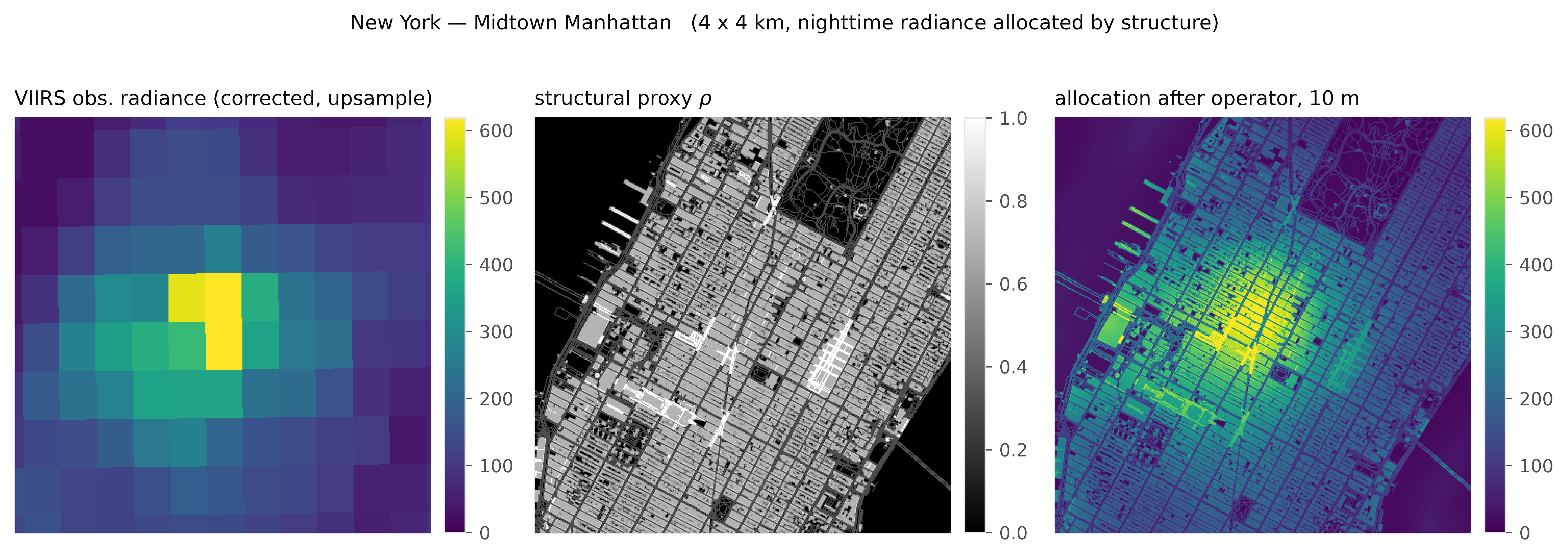
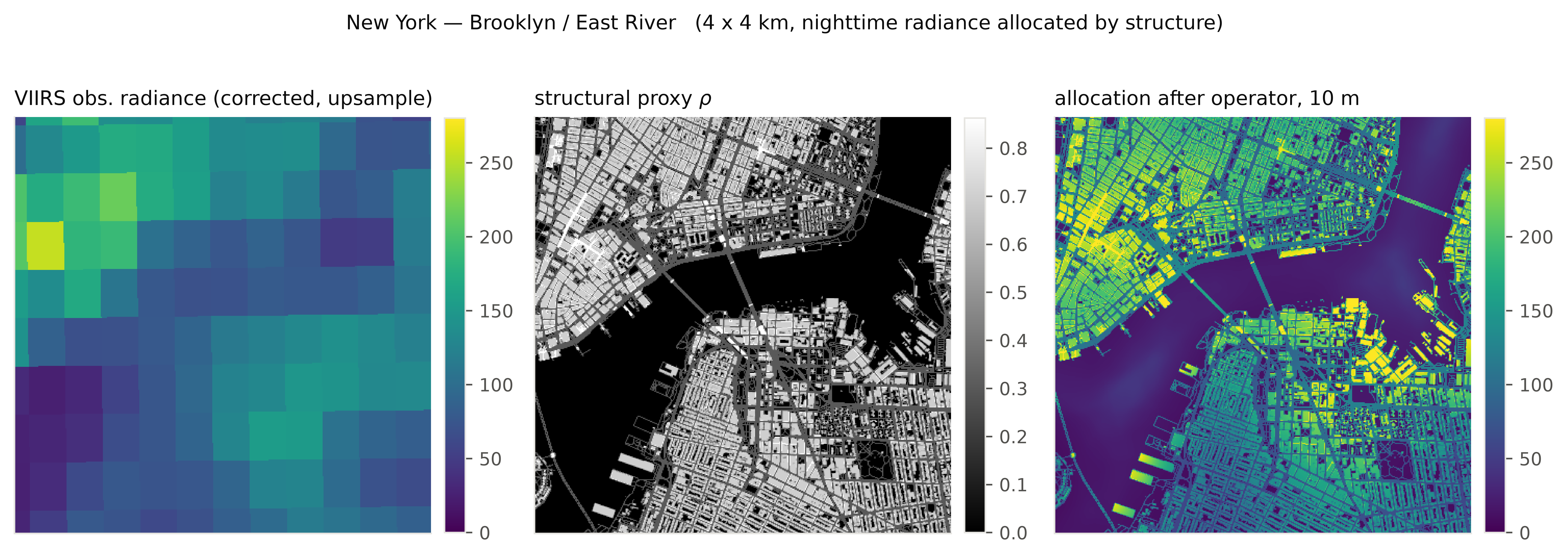
"""Triptych: coarse observation -> structural proxy -> allocation."""
def triptych(city: str, site_key: str, half_km: float = 2.0):
    label, lat, lon = SITES[city][site_key]
    d = cutout(ARTIFACTS[f"direct_{city}"], 1, lat, lon, half_km)
    rho = structure_cutout(city, 3, lat, lon, half_km)   # built_form_base_proxy
    a = cutout(ARTIFACTS[f"primary_{city}"], 1, lat, lon, half_km)

    vmax = float(np.nanpercentile(np.concatenate([d.ravel(), a.ravel()]), 99.0))
    fig, axes = plt.subplots(1, 3, figsize=(11, 3.9))
    for ax, arr, title, cmap, vm in [
        (axes[0], d, "VIIRS obs. radiance (corrected, upsample)", "viridis", vmax),
        (axes[1], rho, "structural proxy $\\rho$", "gray",
         float(np.nanpercentile(rho, 99.0))),
        (axes[2], a, "allocation after operator, 10 m", "viridis", vmax),
    ]:
        im = ax.imshow(arr, cmap=cmap, vmin=0, vmax=vm, interpolation="nearest")
        ax.set_title(title)
        ax.set_xticks([]); ax.set_yticks([])
        fig.colorbar(im, ax=ax, fraction=0.046, pad=0.03)
    fig.suptitle(f"{CITY_LABEL[city]} — {label}   ({half_km*2:.0f} x {half_km*2:.0f} km, "
                 "nighttime radiance allocated by structure)", x=0.5, y=1.02, fontsize=10, color=INK)
    fig.tight_layout()
    plt.savefig(SAVEFIG_PATH / f'tryptych_{city}_{site_key}.png', dpi=600, bbox_inches='tight')
    plt.close(fig)


triptych("usa_new_york", "dense")
triptych("usa_new_york", "water")
/tmp/ipykernel_4640/2247567552.py:14: DeprecationWarning: Setting the shape on a NumPy array has been deprecated in NumPy 2.5.
As an alternative, you can create a new view using np.reshape (with copy=False if needed).
  return src.read(index, window=win, masked=False)
triptych("india_delhi", "dense")
triptych("india_delhi", "water")
/tmp/ipykernel_4640/2247567552.py:14: DeprecationWarning: Setting the shape on a NumPy array has been deprecated in NumPy 2.5.
As an alternative, you can create a new view using np.reshape (with copy=False if needed).
  return src.read(index, window=win, masked=False)
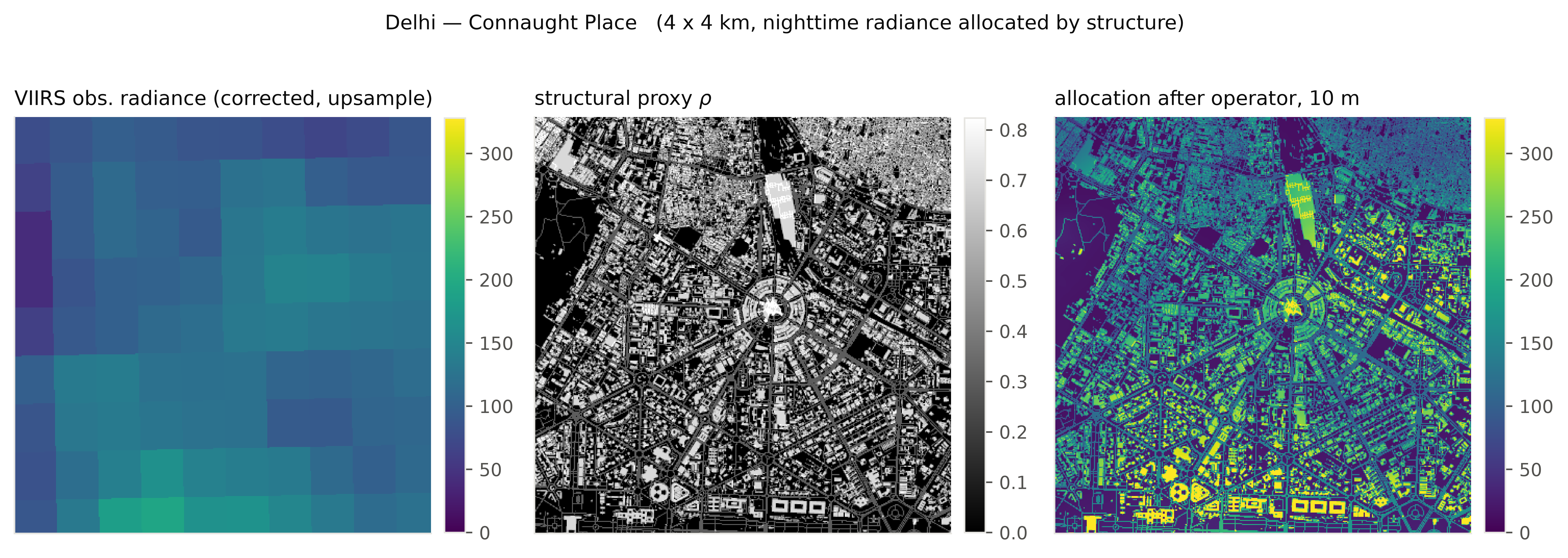
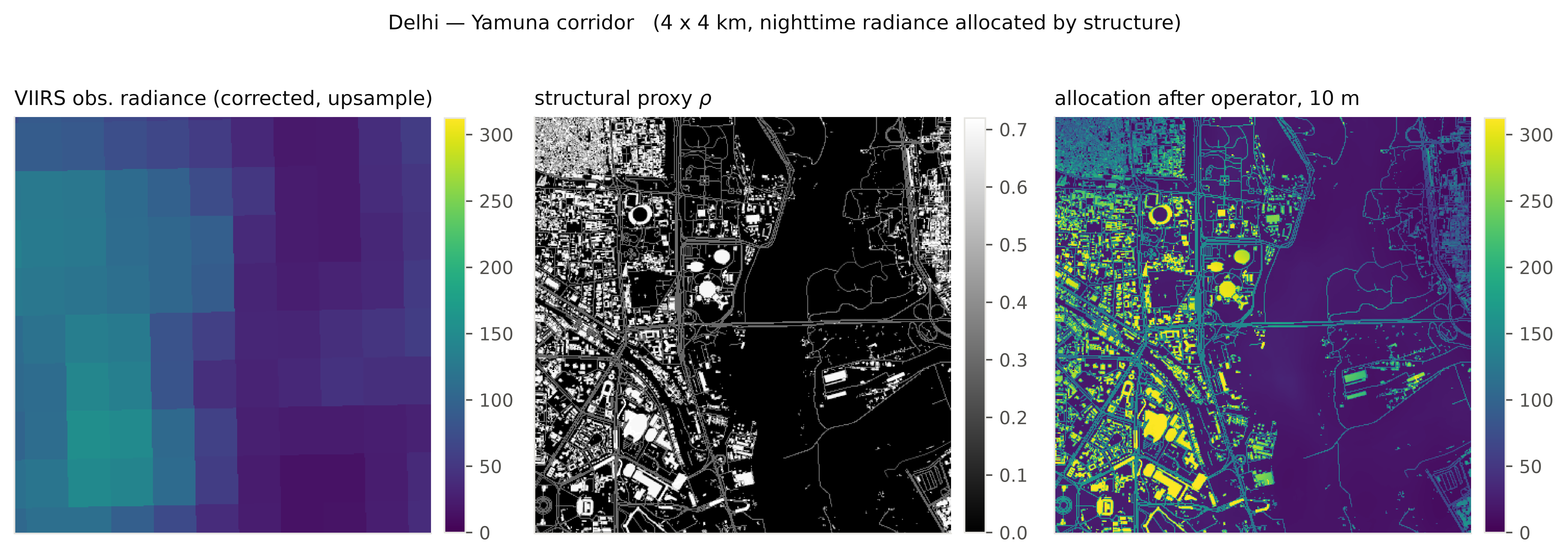
The center panel is doing all the work, whih is a source of concern. The allocation is sharp because $\rho$ is sharp, therefore it inherits the geometry of the building and road layers, not of the light. Where mapped structure and actual lighting coincide, that sharpness is informative. Where they don't, it is confident and wrong, with no internal signal distinguishing the two cases. The sections that follow address this.
A failure cutout
Parks and forest are the honest adversarial case: real VIIRS radiance is present (spill from surrounding streets, atmospheric halo), mapped structure is near-zero, so the operator must push that radiance somewhere.
"""Failure cutout: low proxy support, with the diagnostic bands that flag it."""
def failure_panel(city: str, half_km: float = 2.5):
    label, lat, lon = SITES[city]["failure"]
    panels = [
        (cutout(ARTIFACTS[f"direct_{city}"], 1, lat, lon, half_km),
         "direct upsample (observation)", "viridis", None),
        (cutout(ARTIFACTS[f"primary_{city}"], 1, lat, lon, half_km),
         "allocation", "viridis", None),
        (structure_cutout(city, 3, lat, lon, half_km),
         "proxy $\\rho$", "gray", None),
        (cutout(ARTIFACTS[f"primary_{city}"], 2, lat, lon, half_km),
         "band 2: reaggregation residual", "RdBu_r", "sym"),
        (cutout(ARTIFACTS[f"primary_{city}"], 1, lat, lon, half_km)
         - cutout(ARTIFACTS[f"direct_{city}"], 1, lat, lon, half_km),
         "allocation - direct: where radiance moved", "RdBu_r", "sym"),
        (cutout(ARTIFACTS[f"trust_{city}"], 1, lat, lon, half_km),
         "trust band: allocation gain", "RdBu_r", (0, 2)),
    ]
    fig, axes = plt.subplots(2, 3, figsize=(11, 6.6))
    for ax, (arr, title, cmap, scale) in zip(axes.ravel(), panels):
        if scale == "sym":
            lim = float(np.nanpercentile(np.abs(arr), 99))
            im = ax.imshow(arr, cmap=cmap, vmin=-lim, vmax=lim, interpolation="nearest")
        elif isinstance(scale, tuple):
            im = ax.imshow(arr, cmap=cmap, vmin=scale[0], vmax=scale[1], interpolation="nearest")
        else:
            im = ax.imshow(arr, cmap=cmap, vmin=0,
                           vmax=float(np.nanpercentile(arr, 99)), interpolation="nearest")
        ax.set_title(title); ax.set_xticks([]); ax.set_yticks([])
        fig.colorbar(im, ax=ax, fraction=0.046, pad=0.03)
    fig.suptitle(f"{CITY_LABEL[city]} — {label}: the operator's hardest honest case",
                 x=0.5, y=1.00, fontsize=10, color=INK)
    fig.tight_layout()
    plt.savefig(SAVEFIG_PATH / f'failure_panel_{city}.png', dpi=600, bbox_inches='tight')
    plt.close(fig)

failure_panel("usa_new_york")
/tmp/ipykernel_4640/2247567552.py:14: DeprecationWarning: Setting the shape on a NumPy array has been deprecated in NumPy 2.5.
As an alternative, you can create a new view using np.reshape (with copy=False if needed).
  return src.read(index, window=win, masked=False)
failure_panel("india_delhi")
/tmp/ipykernel_4640/2247567552.py:14: DeprecationWarning: Setting the shape on a NumPy array has been deprecated in NumPy 2.5.
As an alternative, you can create a new view using np.reshape (with copy=False if needed).
  return src.read(index, window=win, masked=False)
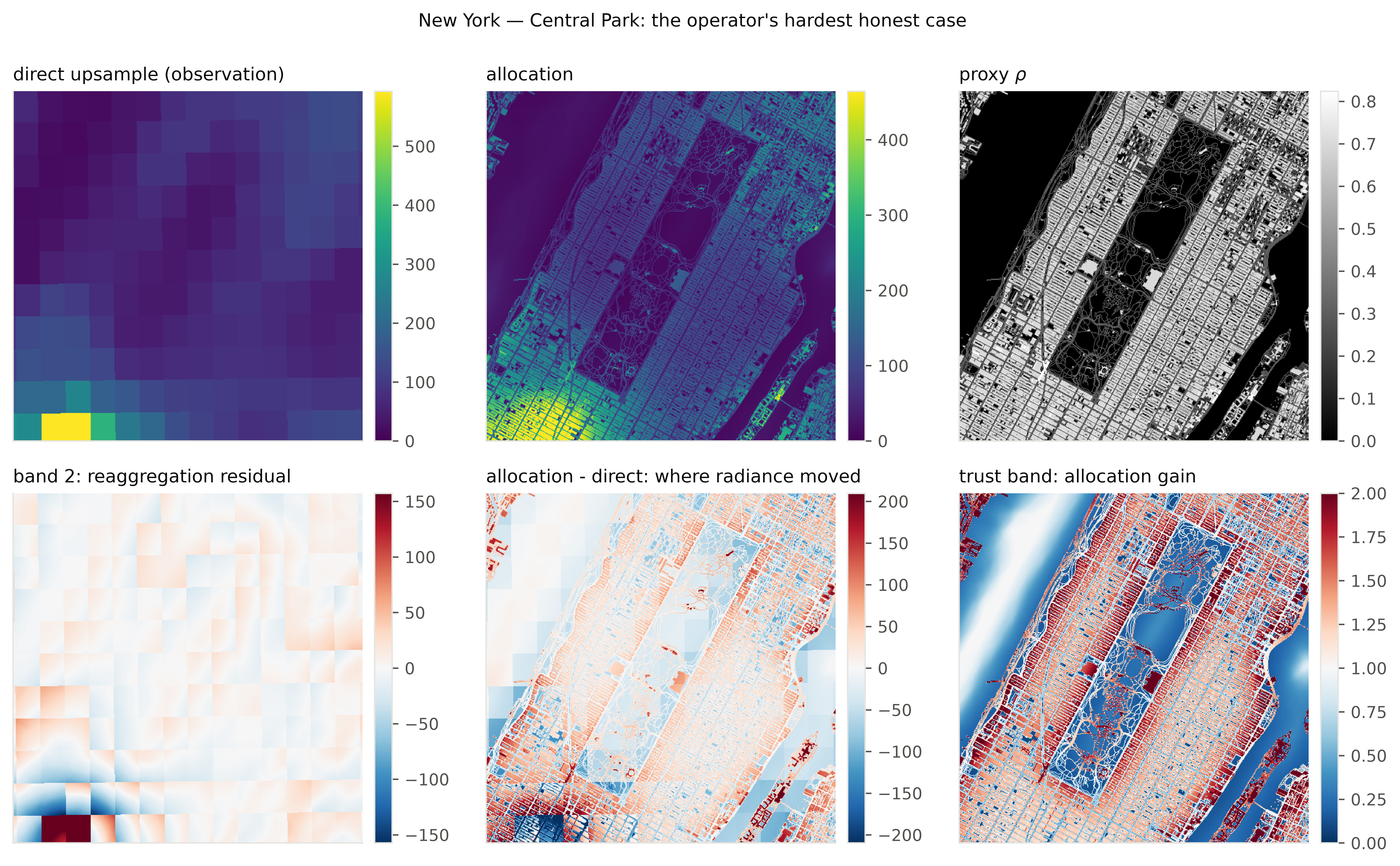
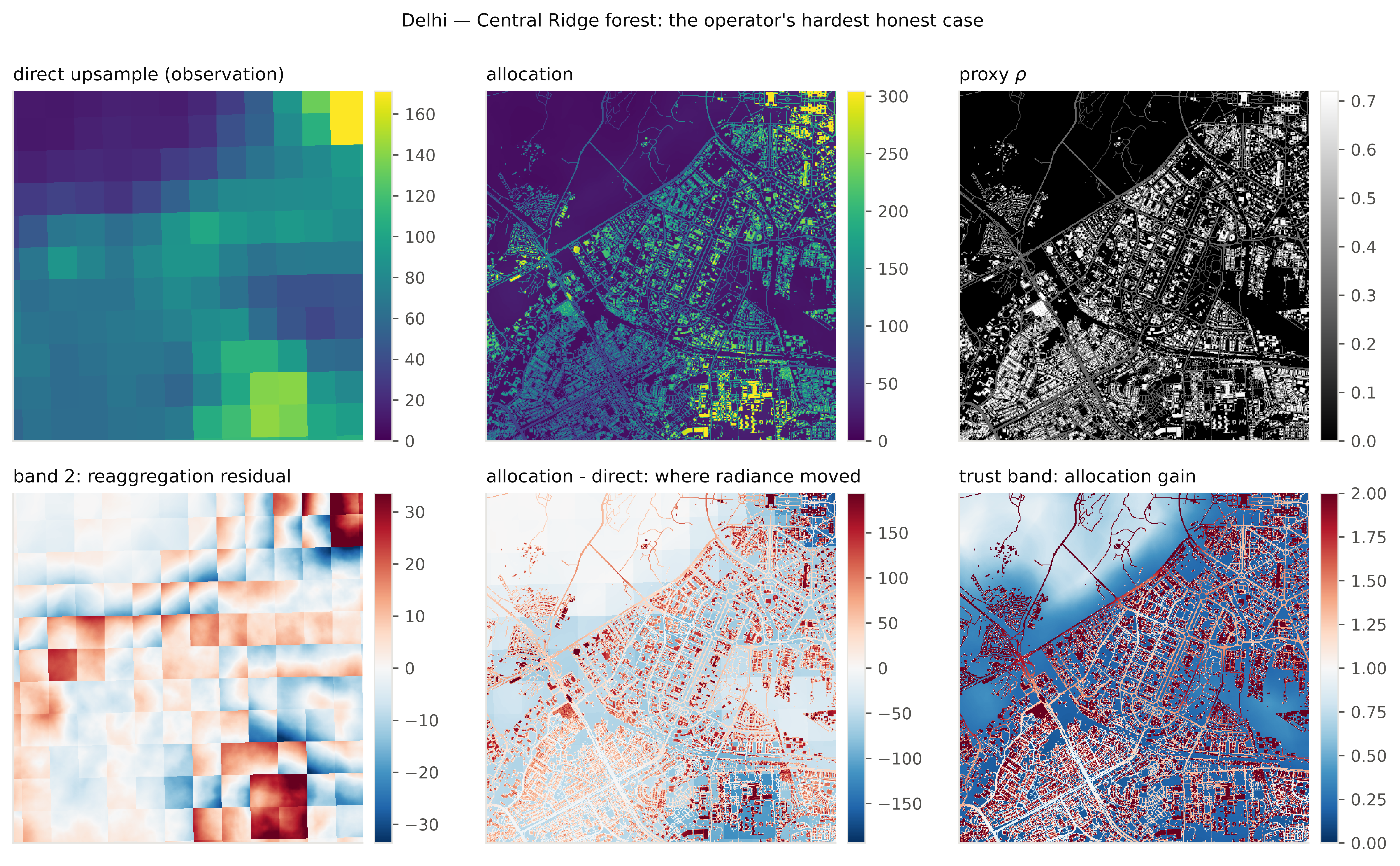
Read the bottom row left to right.
The reaggregation residual (bottom left) is visibly blocky as it inherits the coarse cell geometry, because that is the scale at which local gain fails to close. It is largest where the scene is most heterogeneous within a cell.
The allocation − direct panel (bottom center) is the movement map: red where the operator added radiance relative to the raw observation, blue where it removed it. Parks, water, and rail corridors go blue; building footprints and street corridors go red. This shows what the operator does.
The allocation gain (bottom right) is the same geometry computed without ever touching radiance proxy and kernel only. It goes below 1 (blue) across the park and the water, meaning the operator will move radiance out of those pixels onto surrounding structure. Section 8a shows that this direction of adjustment is the one that measurably helps, and that the opposite direction is the one that hurts.
6. Gate 0: does the prior track the observation at all?
Before implementing the export pipeline, each proxy is aggregated to the VIIRS support and correlated with the observed median. This is a screening gate. It can reject a nonsensical allocation hypothesis; it cannot validate a sensible one, and passing it says nothing about within-pixel behavior.
Strict QA, frozen cohort, v3 artifacts (grid + halo + datatake mosaic + S2 support threshold).
"""Gate 0 v3 summary tables."""
g0_bf = pd.read_csv(ARTIFACTS["gate0_builtform"])
g0_s2 = pd.read_csv(ARTIFACTS["gate0_s2"])
print("built-form primary:")
display(g0_bf)
print("S2-only ablation:")
display(g0_s2)

regen = load_json(ARTIFACTS["gate0_regen"])
print("figure regeneration record (deviation #2 from section 4):")
print(json.dumps({k: v for k, v in regen.items() if not isinstance(v, (list, dict))},
                 indent=2))
built-form primary:
| city_id | allocation_proxy | sample_count | input_sample_count | excluded_s2_coarse_support_fraction | minimum_s2_coarse_support_fraction | block_count | citywide_spearman | block_aggregate_spearman | block_mean_spearman | ... | continuous_resampling | categorical_resampling | s2_composite_decision_id | s2_composite_method | s2_minimum_common_valid_observations | s2_coarse_support_decision_id | gate0_aggregation_halo_m | gate0_status | overture_release | built_form_temporal_semantics | |
|---|---|---|---|---|---|---|---|---|---|---|---|---|---|---|---|---|---|---|---|---|---|
| 0 | usa_new_york | built_form_primary | 15335 | 15335 | 0.0 | 0.9 | 121 | 0.811875 | 0.826067 | 0.826067 | ... | bilinear | nearest | S2-COMPOSITE-001 | index_of_bandwise_temporal_medians_after_datat... | 5 | S2-SUPPORT-001 | 1000 | current_corrected_rerun | 2026-07-22.0 | contemporary_structural_proxy_used_to_allocate... |
| 1 | india_delhi | built_form_primary | 13280 | 13280 | 0.0 | 0.9 | 121 | 0.761388 | 0.900982 | 0.900982 | ... | bilinear | nearest | S2-COMPOSITE-001 | index_of_bandwise_temporal_medians_after_datat... | 5 | S2-SUPPORT-001 | 1000 | current_corrected_rerun | 2026-07-22.0 | contemporary_structural_proxy_used_to_allocate... |
2 rows × 40 columns
S2-only ablation:
| city_id | allocation_proxy | sample_count | input_sample_count | excluded_s2_coarse_support_fraction | minimum_s2_coarse_support_fraction | block_count | citywide_spearman | block_aggregate_spearman | block_mean_spearman | ... | vnp_quality_decision_id | resampling_decision_id | continuous_resampling | categorical_resampling | s2_composite_decision_id | s2_composite_method | s2_minimum_common_valid_observations | s2_coarse_support_decision_id | gate0_aggregation_halo_m | gate0_status | |
|---|---|---|---|---|---|---|---|---|---|---|---|---|---|---|---|---|---|---|---|---|---|
| 0 | usa_new_york | s2_only_ablation | 14963 | 15335 | 0.024258 | 0.9 | 121 | 0.783180 | 0.811195 | 0.811195 | ... | VNP-QA-001 | RESAMPLE-001 | bilinear | nearest | S2-COMPOSITE-001 | index_of_bandwise_temporal_medians_after_datat... | 5 | S2-SUPPORT-001 | 1000 | current_corrected_rerun |
| 1 | india_delhi | s2_only_ablation | 13280 | 13280 | 0.000000 | 0.9 | 121 | 0.437784 | 0.575816 | 0.575816 | ... | VNP-QA-001 | RESAMPLE-001 | bilinear | nearest | S2-COMPOSITE-001 | index_of_bandwise_temporal_medians_after_datat... | 5 | S2-SUPPORT-001 | 1000 | current_corrected_rerun |
2 rows × 38 columns
figure regeneration record (deviation #2 from section 4):
{
  "artifact_version": "v3_qa_grid_halo_datatake_support",
  "created_at_utc": "2026-07-30T15:53:47.609707+00:00",
  "defect_closed": "ARTIFACT-PROVENANCE-001",
  "schema_version": 1,
  "source_policy": "saved v3 samples and v3 summary tables only"
}
"""The regenerated v3 Gate 0 panels."""
from matplotlib.image import imread

g0_dir = VAL / "gate0/v3_qa_grid_halo_datatake_support"
panels = [
    ("usa_new_york_built_form_gate0.png", "New York: built form"),
    ("india_delhi_built_form_gate0.png", "Delhi: built form"),
    ("usa_new_york_s2_only_gate0.png", "New York: S2 only"),
    ("india_delhi_s2_only_gate0.png", "Delhi: S2 only"),
]
fig, axes = plt.subplots(2, 2, figsize=(12, 9))
for ax, (fn, title) in zip(axes.ravel(), panels):
    path = g0_dir / fn
    if path.exists():
        ax.imshow(imread(path))
        ax.set_title(title)
    ax.axis("off")
fig.tight_layout()
plt.savefig(SAVEFIG_PATH / "gate0-panels.png", dpi=300, bbox_inches="tight")
plt.close(fig)
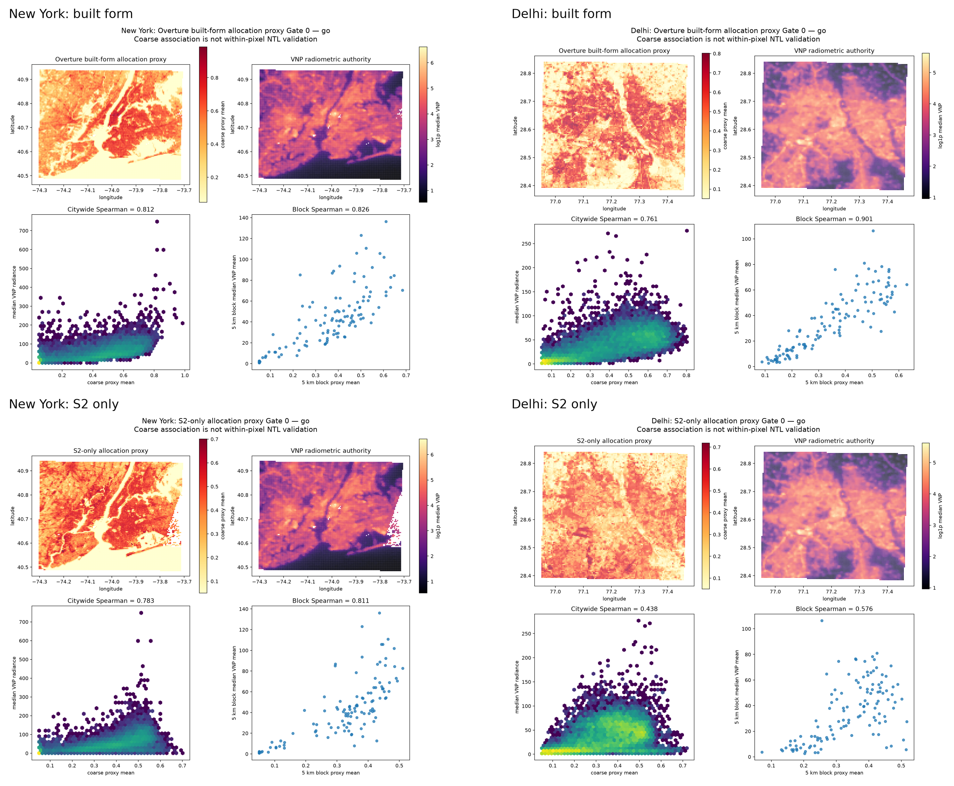
Delhi S2-Only is a confident miss (bad)
Look at the Delhi S2-only panel. The relationship between proxy and radiance is not monotone, it is mound-shaped: radiance rises with the proxy, peaks, and then turns down in the upper proxy range. The reason is that the Sentinel images are taken pre-monsoon. Bare soil and the exposed Yamuna channel are spectrally bright, low in vegetation index, and not water, which the S2-only proxy incorrectly reads as built-up area.
Two things about how this was caught matter more than the finding itself.
First, the Gate 0 decision rule did not test for this. It required positive citywide, block, and detrended Spearman correlations, and Delhi S2-only passed all three (0.438 / 0.576 / 0.499) while being badly non-monotone in the bright tail. A mound-shaped association clears every positive-correlation threshold you can write. The word "monotone" in the S2-only proxy definition described how the proxy was constructed, never its empirical relationship to radiance.
Second, this is recorded as GATE0-MONOTONICITY-001 i.e. a rule gap, discovered
downstream at Gate 2, with no retrospective threshold change and no retroactive
proxy pruning.
Delhi S2-only is followed to its conclusion in section 8f.
7. Held-out validation design
Validation is a key question here.
How do you test an allocation operator when you have no independent fine-grid nighttime measurement? In the future, I plan to compare this method with hi-res imagery, such as produced by SDBSAT-1. So I"m not actually able to test the validity of the 10m field.
HOwever, I can test whether the structural prior predicts radiance it was never allowed to see, at the coarse scale where ground truth exists. i.e. a hold-out validation.
Procedure. Partition native VNP cells into 5 spatially-blocked folds. For a held-out fold: remove its radiance, estimate the local allocation gain from the retained neighborhood only, predict the held-out cell, and compare with the untouched observation. The baseline is neighbors-only inverse-distance-squared interpolation using the identical eligible training cells.
The buffer. Held-out folds are buffered at a distance so the target's own signal cannot leak back through nearby observed cells. VIIRS is a convolution, so a neighboring cell contains PSF-mediated signal from the target. The primary buffer is 2550 m: the registered four-sigma truncation radius of the widest declared Gaussian sensitivity (1500 m FWHM). It is derived from the kernel family, not chosen as a round number. 1500 m and 2000 m run as sensitivities.
The property that makes the buffer interpretable. Widening the buffer removes eligible neighbors, not targets. The target set is identical at every buffer. So the three buffers are not independent resamples, rather they are the same cells predicted from progressively more distant information. Section 8b uses this.
"""Held-out design: target and neighbor retention across buffers (broad QA)."""
ret = pd.read_csv(ARTIFACTS["heldout_broad_retain"])
print("columns:", list(ret.columns))
display(ret.head(20))
columns: ['city_id', 'proxy', 'buffer_m', 'buffer_role', 'fold', 'target_count', 'retained_target_count', 'retained_target_fraction', 'median_nearest_neighbor_distance_m', 'median_distance_to_block_edge_m']
| city_id | proxy | buffer_m | buffer_role | fold | target_count | retained_target_count | retained_target_fraction | median_nearest_neighbor_distance_m | median_distance_to_block_edge_m | |
|---|---|---|---|---|---|---|---|---|---|---|
| 0 | usa_new_york | built_form_primary | 1500.0 | sensitivity | all | 15335 | 15335 | 1.0 | 1556.464369 | 731.536887 |
| 1 | usa_new_york | built_form_primary | 1500.0 | sensitivity | 0 | 3154 | 3154 | 1.0 | 1556.469038 | 714.046400 |
| 2 | usa_new_york | built_form_primary | 1500.0 | sensitivity | 1 | 3095 | 3095 | 1.0 | 1556.467985 | 718.179774 |
| 3 | usa_new_york | built_form_primary | 1500.0 | sensitivity | 2 | 3017 | 3017 | 1.0 | 1556.484332 | 766.682052 |
| 4 | usa_new_york | built_form_primary | 1500.0 | sensitivity | 3 | 2994 | 2994 | 1.0 | 1556.446582 | 799.197863 |
| 5 | usa_new_york | built_form_primary | 1500.0 | sensitivity | 4 | 3075 | 3075 | 1.0 | 1556.455602 | 729.206659 |
| 6 | usa_new_york | built_form_primary | 2000.0 | sensitivity | all | 15335 | 15335 | 1.0 | 2113.592303 | 731.536887 |
| 7 | usa_new_york | built_form_primary | 2000.0 | sensitivity | 0 | 3154 | 3154 | 1.0 | 2113.895053 | 714.046400 |
| 8 | usa_new_york | built_form_primary | 2000.0 | sensitivity | 1 | 3095 | 3095 | 1.0 | 2113.663482 | 718.179774 |
| 9 | usa_new_york | built_form_primary | 2000.0 | sensitivity | 2 | 3017 | 3017 | 1.0 | 2113.420146 | 766.682052 |
| 10 | usa_new_york | built_form_primary | 2000.0 | sensitivity | 3 | 2994 | 2994 | 1.0 | 2113.440071 | 799.197863 |
| 11 | usa_new_york | built_form_primary | 2000.0 | sensitivity | 4 | 3075 | 3075 | 1.0 | 2113.649075 | 729.206659 |
| 12 | usa_new_york | built_form_primary | 2550.0 | primary | all | 15335 | 15335 | 1.0 | 2554.181578 | 731.536887 |
| 13 | usa_new_york | built_form_primary | 2550.0 | primary | 0 | 3154 | 3154 | 1.0 | 2554.209982 | 714.046400 |
| 14 | usa_new_york | built_form_primary | 2550.0 | primary | 1 | 3095 | 3095 | 1.0 | 2554.139753 | 718.179774 |
| 15 | usa_new_york | built_form_primary | 2550.0 | primary | 2 | 3017 | 3017 | 1.0 | 2554.167884 | 766.682052 |
| 16 | usa_new_york | built_form_primary | 2550.0 | primary | 3 | 2994 | 2994 | 1.0 | 2554.177071 | 799.197863 |
| 17 | usa_new_york | built_form_primary | 2550.0 | primary | 4 | 3075 | 3075 | 1.0 | 2554.205352 | 729.206659 |
| 18 | usa_new_york | s2_only_ablation | 1500.0 | sensitivity | all | 15335 | 15335 | 1.0 | 1556.464369 | 731.536887 |
| 19 | usa_new_york | s2_only_ablation | 1500.0 | sensitivity | 0 | 3154 | 3154 | 1.0 | 1556.469038 | 714.046400 |
"""Confirm the design property: identical target counts across buffers."""
hb = pd.read_csv(ARTIFACTS["heldout_broad"])
overall = hb[(hb.fold.astype(str) == "all") & (hb.radiance_decile.astype(str) == "all")]
tgt = (overall[overall.method == "neighbors_only_prediction"]
       .pivot_table(index="city_id", columns="buffer_m", values="sample_count"))
display(tgt)
constant = tgt.nunique(axis=1).eq(1).all()
print(f"target set identical across all three buffers: {constant}")
print("=> differences across buffers measure distance dependence, not resampling.")
| buffer_m | 1500.0 | 2000.0 | 2550.0 |
|---|---|---|---|
| city_id | |||
| india_delhi | 13280.0 | 13280.0 | 13280.0 |
| usa_new_york | 15335.0 | 15335.0 | 15335.0 |
target set identical across all three buffers: True
=> differences across buffers measure distance dependence, not resampling.
8. Results
8a. The gain asymmetry: lead with the mechanism
The most informative result in the experiment is not actually the error reduction. It is a radiance-blind diagnostic: stratify held-out cells by allocation gain, which is to say the target's proxy divided by its weighted training-neighbor proxy, into preregistered strata below 0.8, 0.8–1.25, and at or above 1.25. Gain is computed from proxy and kernel only. Therefore radiance cancels out.
Then ask, within each stratum, whether the structural prediction beat the neighbors-only baseline in estimating where radiance was in the dropped/held-out cell.
"""Gain asymmetry, broad QA, primary 2550 m buffer."""
gb = pd.read_csv(ARTIFACTS["heldout_broad_gain"])
gp = gb[(gb.buffer_m == 2550)].copy()
gp["city"] = gp.city_id.map(CITY_LABEL)

tbl = gp.pivot_table(index=["city", "proxy"], columns="gain_stratum",
                     values="structural_minus_neighbors_absolute_error")
tbl = tbl[["<0.8", "0.8-1.25", ">=1.25"]]
display(tbl.round(3))
print("Negative = structural prediction beats neighbors-only. Units: radiance (nW/cm2/sr).")
| gain_stratum | <0.8 | 0.8-1.25 | >=1.25 | |
|---|---|---|---|---|
| city | proxy | |||
| Delhi | built_form_primary | -5.956 | 0.459 | 2.113 |
| s2_only_ablation | -3.482 | 0.730 | 3.407 | |
| New York | built_form_primary | -10.253 | -0.169 | 2.127 |
| s2_only_ablation | -10.941 | -0.275 | 0.501 |
Negative = structural prediction beats neighbors-only. Units: radiance (nW/cm2/sr).
"""Figure: gain asymmetry as small multiples.

Small multiples rather than grouped bars: the message is that all four
combinations share one shape, and color is already spent on polarity
(improve/harm), so series identity needs its own panel rather than a
fifth hue.
"""
strata = ["<0.8", "0.8-1.25", ">=1.25"]
combos = [(c, p) for c in ["usa_new_york", "india_delhi"]
          for p in ["built_form_primary", "s2_only_ablation"]]

lim = float(np.abs(gp.structural_minus_neighbors_absolute_error).max()) * 1.28
fig, axes = plt.subplots(1, 4, figsize=(11, 3.9), sharey=True)
xs = np.arange(len(strata))

for ax, (city, proxy) in zip(axes, combos):
    sub = gp[(gp.city_id == city) & (gp.proxy == proxy)].set_index("gain_stratum")
    vals = np.array([sub.loc[s, "structural_minus_neighbors_absolute_error"]
                     for s in strata])
    colors = [COLOR["improve"] if v < 0 else COLOR["harm"] for v in vals]
    ax.bar(xs, vals, 0.66, color=colors, edgecolor="white", linewidth=1.4)
    for x, v in zip(xs, vals):
        ax.annotate(f"{v:+.1f}", (x, v), ha="center",
                    va="top" if v < 0 else "bottom",
                    xytext=(0, -4 if v < 0 else 4), textcoords="offset points",
                    fontsize=8, color=INK_2)
    ax.axhline(0, color=INK, lw=1.0)
    ax.set_xticks(xs)
    ax.set_xticklabels(["< 0.8", "0.8-\n1.25", ">= 1.25"], fontsize=8)
    ax.set_title(f"{CITY_LABEL[city]}\n{'built form' if 'built' in proxy else 'S2 only'}",
                 fontsize=9)
    ax.set_ylim(-lim, lim)
    ax.grid(axis="y"); ax.set_axisbelow(True)
    ax.spines["left"].set_visible(False)
    ax.tick_params(axis="y", length=0)

axes[0].set_ylabel("structural MAE - neighbors MAE")
handles = [mpl.patches.Patch(color=COLOR["improve"], label="structural prediction better"),
           mpl.patches.Patch(color=COLOR["harm"], label="structural prediction worse")]
fig.legend(handles=handles, loc="lower center", ncol=2, fontsize=8,
           bbox_to_anchor=(0.5, -0.06))
fig.suptitle("Downweighting helps a lot. Upweighting hurts. Same shape in all four "
             "city x proxy combinations.\nx axis: allocation gain stratum "
             "(radiance-blind, computed from structure proxy and kernel only).",
             x=0.5, y=1.08, fontsize=9.5, color=INK, ha="center")
fig.tight_layout()
plt.savefig(SAVEFIG_PATH / f'gain_asymmetry.png', dpi=600, bbox_inches='tight')
plt.close(fig)
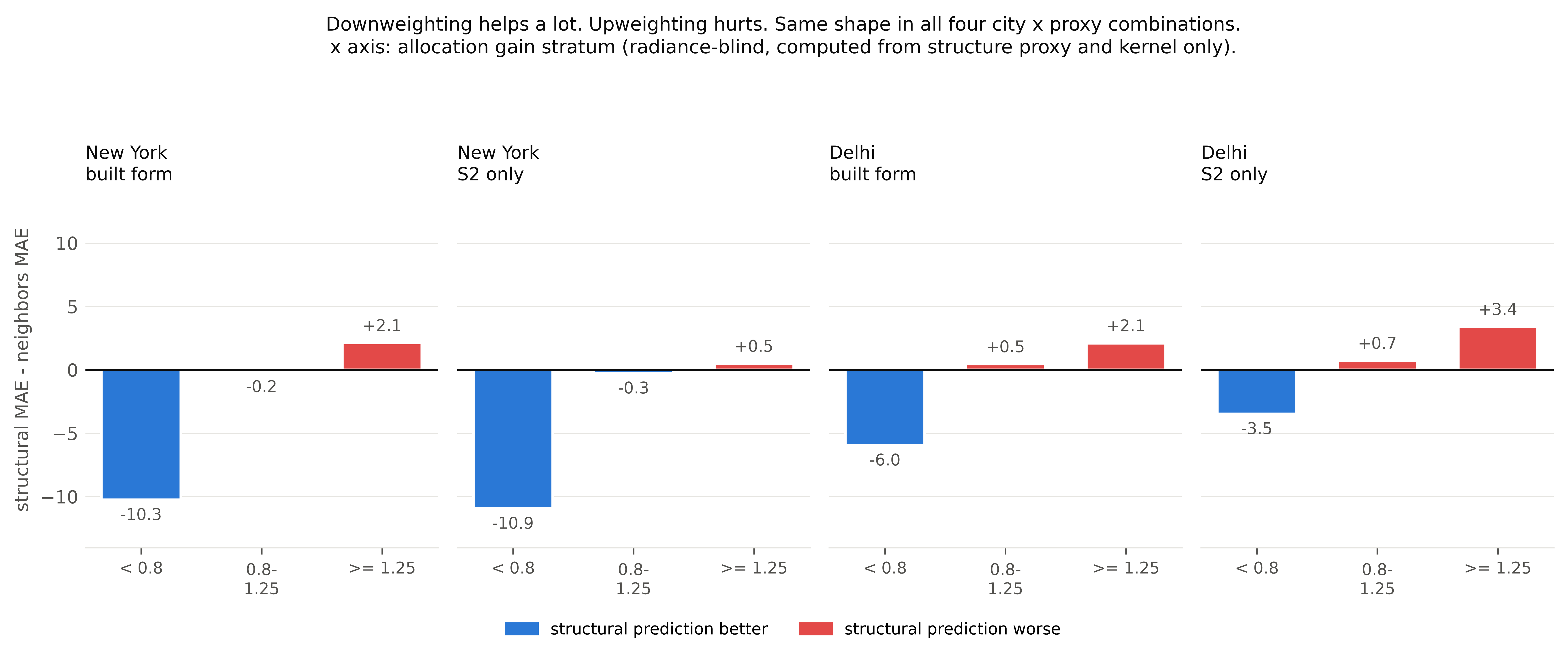
Monotone in the same direction in all four combinations, and as per section 8b, stable across all three buffers. The interpretation:
Absence of built form is a near-hard constraint on absence of light. Presence of built form is a weak constraint on its magnitude.
Structure tells you reliably where light isn't. It tells you much less about how bright the lit places are. Which is what you would expect if mapped structure captures where lighting infrastructure can physically exist, but not its density, lamp power, usage, or commercial intensity.
One practical way to think about this is that if there is no structure (park, water), the method correctly constrains light. But where there is structure, it could be a dense cluster of light buildings (time square) or a bunch of dark warehouses and this ambiguity means structure alone does not do as well to show the magnitude of light. Given the use of nighttime lights to assess economic activity, this is a true challenge to using this method to infer activfity at a fine-grained spatial resolution. Such inference requires higher resolution observation or maybe additional data about the structure type or use.
Is this just noise?
If $\rho$ is noisy, then gain is a ratio of noisy quantities, and extreme gain values are where the noise is largest, so of course error is worse there. No structural interpretation needed.
That objection makes a testable prediction. Pure multiplicative ratio noise is symmetric in log-gain: it should degrade the low and high strata comparably. The observed pattern is strongly asymmetric. Simulate it.
"""Noise simulation: can ratio noise alone reproduce the observed pattern?

Design mirrors the actual held-out estimator, at the coarse-cell scale where it
operates. Known truth L; a proxy rho = L * lognormal noise -- i.e. a proxy whose
ONLY defect is multiplicative noise, with no structural information missing.
Gain, strata, and the structural predictor are computed exactly as in the real
run. The kernel is held fixed; only rho is perturbed.

Second arm: a heavy right-tailed truth field, testing whether proxy tail shape
(built form is a sqrt-transformed building fraction plus saturating road density)
is a competing explanation.

Errors are reported as PERCENT CHANGE relative to the neighbors-only baseline in
the same stratum, so simulated and observed are on a common scale.
"""
from scipy import ndimage as _ndi

rng = np.random.default_rng(20260803)
N_CELLS = 140


def smooth_noise(n, scale, rng):
    a = _ndi.gaussian_filter(rng.normal(size=(n, n)), scale, mode="reflect")
    return a / a.std()


def neighbor_mean(c):
    ker = np.array([[0, 1, 0], [1, 0, 1], [0, 1, 0]], dtype=float)
    return _ndi.convolve(c, ker / ker.sum(), mode="reflect")


def simulate(arm: str, sigma: float, n_rep: int = 8) -> pd.DataFrame:
    """Return the two summary statistics the real run also reports:
    overall percent change in MAE vs the neighbors-only baseline, and the
    dispersion of the gain field (share of cells outside the middle stratum).
    """
    rows = []
    for _ in range(n_rep):
        base = np.exp(1.1 * smooth_noise(N_CELLS, 4.0, rng))
        if arm == "heavy-tailed proxy":
            base = base ** 2.2
        L = 20.0 + 180.0 * base / base.mean()
        rho = L * np.exp(sigma * smooth_noise(N_CELLS, 0.8, rng))

        nb_L = neighbor_mean(L)
        gain = rho / np.maximum(neighbor_mean(rho), 1e-9)
        structural = nb_L * gain

        err_s, err_n = np.abs(structural - L), np.abs(nb_L - L)
        rows.append({
            "arm": arm, "sigma": sigma,
            "pct_delta": 100 * (err_s.mean() - err_n.mean()) / err_n.mean(),
            "dispersion": 100 * float(((gain < 0.8) | (gain >= 1.25)).mean()),
        })
    return (pd.DataFrame(rows)
            .groupby(["arm", "sigma"], as_index=False)[["pct_delta", "dispersion"]]
            .mean())


SIGMAS = [0.02, 0.05, 0.08, 0.12, 0.16, 0.20, 0.25, 0.30, 0.40, 0.50]
sim = pd.concat([simulate(arm, s) for s in SIGMAS
                 for arm in ("ratio noise only", "heavy-tailed proxy")],
                ignore_index=True)

# observed: same two summary statistics, from the broad-QA held-out run
obs_rows = []
for city in CITIES:
    for proxy in ("built_form_primary", "s2_only_ablation"):
        g = gb[(gb.buffer_m == 2550) & (gb.city_id == city) & (gb.proxy == proxy)]
        n = g.sample_count.sum()
        o = hb[(hb.buffer_m == 2550) & (hb.city_id == city) & (hb.proxy == proxy) &
               (hb.fold.astype(str) == "all") & (hb.radiance_decile.astype(str) == "all")]
        nb_mae = o[o.method == "neighbors_only_prediction"].mae.iloc[0]
        st_mae = o[o.method == "structural_prediction"].mae.iloc[0]
        obs_rows.append({
            "label": f"{CITY_LABEL[city]} {'built form' if 'built' in proxy else 'S2 only'}",
            "proxy": proxy,
            "pct_delta": 100 * (st_mae - nb_mae) / nb_mae,
            "dispersion": 100 * g[g.gain_stratum != "0.8-1.25"].sample_count.sum() / n,
        })
observed = pd.DataFrame(obs_rows)

display(sim.pivot_table(index="sigma", columns="arm",
                        values=["pct_delta", "dispersion"]).round(1))
print("\nOBSERVED:")
display(observed.round(1))
| dispersion | pct_delta | |||
|---|---|---|---|---|
| arm | heavy-tailed proxy | ratio noise only | heavy-tailed proxy | ratio noise only |
| sigma | ||||
| 0.02 | 0.9 | 0.0 | -88.3 | -67.1 |
| 0.05 | 0.9 | 0.0 | -73.4 | -19.6 |
| 0.08 | 1.0 | 0.0 | -49.5 | 27.4 |
| 0.12 | 1.4 | 0.0 | -31.9 | 107.3 |
| 0.16 | 2.2 | 0.3 | -5.2 | 167.0 |
| 0.20 | 3.9 | 1.5 | 11.7 | 244.3 |
| 0.25 | 7.4 | 5.0 | 42.1 | 305.5 |
| 0.30 | 12.7 | 10.3 | 65.0 | 383.0 |
| 0.40 | 24.0 | 22.2 | 144.0 | 574.9 |
| 0.50 | 34.9 | 33.6 | 171.2 | 741.3 |
OBSERVED:
| label | proxy | pct_delta | dispersion | |
|---|---|---|---|---|
| 0 | New York built form | built_form_primary | -14.0 | 54.1 |
| 1 | New York S2 only | s2_only_ablation | -15.7 | 47.3 |
| 2 | Delhi built form | built_form_primary | -10.0 | 63.3 |
| 3 | Delhi S2 only | s2_only_ablation | 1.2 | 50.0 |
Read the two tables together.
A noise-only proxy has a single free parameter, $\sigma$. Turning it up does two things at once: it spreads the gain distribution (dispersion rises) and it destroys accuracy (percent change rises). Those move together, and they cannot be decoupled, so there is no setting that gives you wide gain dispersion and an overall improvement.
The real proxies achieve both simultaneously. They spread gain across ~47–63% of cells outside the middle stratum while reducing overall error by 10–16%. The next figure shows there is no point on the noise-only trajectory anywhere near them.
"""Figure: the noise-only trajectory cannot reach the observed operating point."""
fig, ax = plt.subplots(figsize=(9.2, 5.4))

# shade the quadrant no noise-only proxy can reach
ax.axhspan(-30, 0, xmin=0.0, xmax=1.0, color=BLUE, alpha=0.05, zorder=0)

# Both simulated arms are the SAME model with one assumption changed, so they
# share a hue and separate by line style + marker. This also keeps the on-screen
# palette to categorical slots 1-3 (blue / orange / aqua), the three that clear
# the all-pairs CVD floors -- avoiding the documented orange-yellow failure.
for arm, ls, marker in [("ratio noise only", "-", "o"),
                        ("heavy-tailed proxy", "--", "s")]:
    s = sim[sim.arm == arm].sort_values("sigma")
    ax.plot(s.dispersion, s.pct_delta, color=ORANGE, ls=ls, lw=2, marker=marker,
            ms=5, mec="white", mew=1.0, label=f"simulated: {arm}", zorder=2)

# annotate sigma on one curve only, to the right of the marker
s = sim[sim.arm == "heavy-tailed proxy"].sort_values("sigma")
for _, r in s.iterrows():
    if r.sigma in (0.20, 0.50):
        ax.annotate(f"$\\sigma$={r.sigma:g}", (r.dispersion, r.pct_delta),
                    xytext=(8, -2), textcoords="offset points",
                    fontsize=7.5, color=MUTED, va="center")

for _, r in observed.iterrows():
    ax.scatter([r.dispersion], [r.pct_delta], s=120,
               color=COLOR[r.proxy], edgecolor="white", linewidth=1.6, zorder=4)
    ax.annotate(r.label, (r.dispersion, r.pct_delta), xytext=(0, -13),
                textcoords="offset points", fontsize=8, color=INK_2,
                ha="center", va="top")

ax.axhline(0, color=INK, lw=1.0, zorder=1)
ax.set_xlabel("gain dispersion: cells outside the 0.8-1.25 stratum (%)")
ax.set_ylabel("overall change in MAE vs neighbors-only (%)")
ax.set_title("A noise-only proxy cannot be both widely dispersed and accurate")
ax.set_yscale("symlog", linthresh=25)
ax.set_yticks([-20, 0, 25, 100, 400])
ax.set_yticklabels(["-20  (better)", "0", "+25", "+100", "+400  (worse)"])
ax.set_xlim(-3, 74)
ax.set_ylim(-32, 900)
ax.annotate("observed proxies live in the shaded quadrant:\n"
            "wide gain dispersion AND lower error.\n"
            "No noise level reaches it.",
            (71, 220), fontsize=8.5, color=BLUE, ha="right", va="center",
            linespacing=1.5)
ax.grid(True); ax.set_axisbelow(True)
ax.legend(loc="upper left", fontsize=8)
fig.tight_layout()
plt.savefig(SAVEFIG_PATH / "noise-only-trajectory.png", dpi=300, bbox_inches="tight")
plt.close(fig)
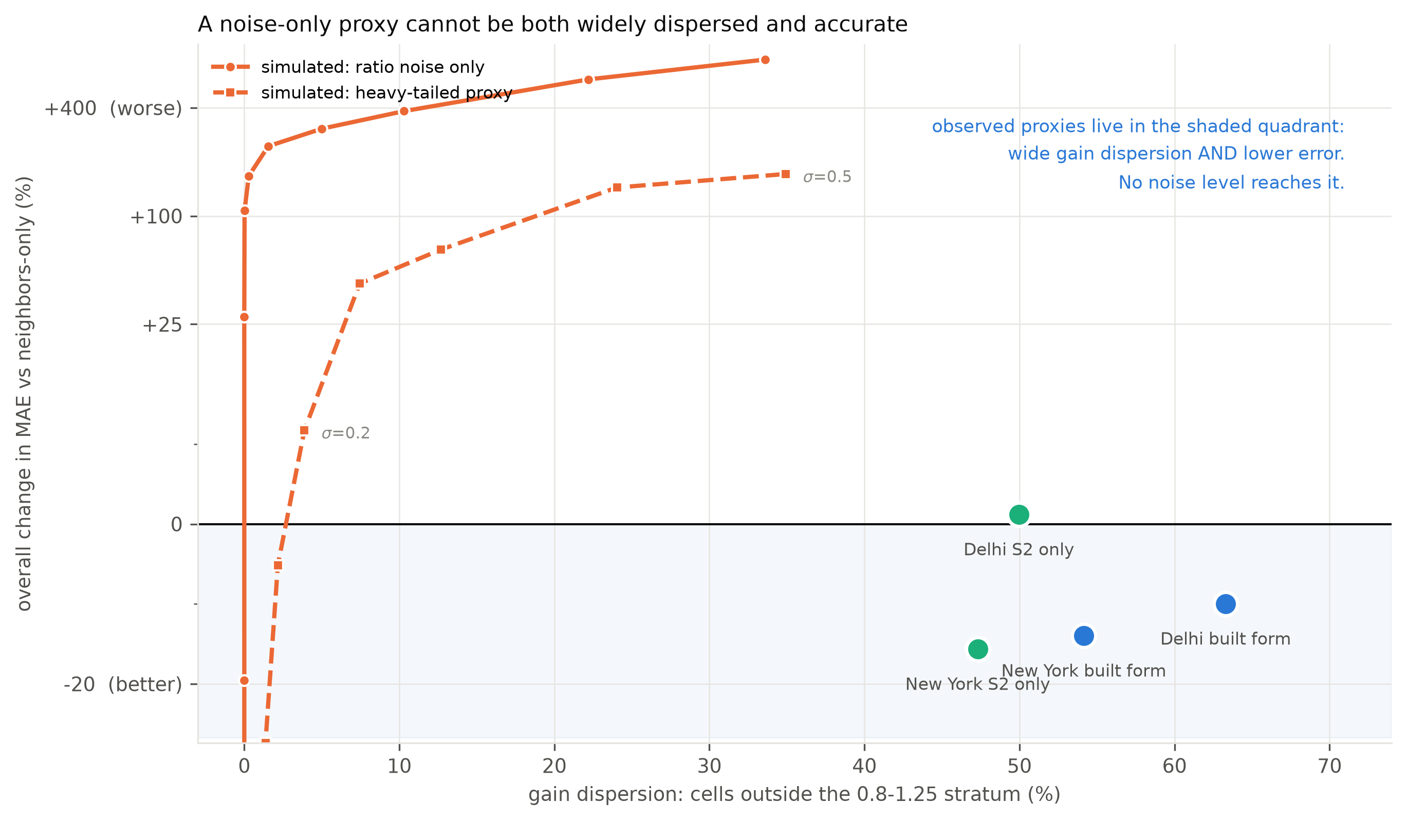
The observed proxies for all 4 city/layer scenarios sit in the lower right: wide gain dispersion, negative error change. The simulated trajectories never enter that quadrant, for any noise level, in either arm. To match the observed dispersion (~54% for New York built form) a noise-only proxy needs $\sigma > 0.5$, where it degrades MAE by well over 100%. To match the observed accuracy it needs $\sigma \approx 0.05$, where gain dispersion is essentially zero.
the gain field is not noise. It carries information that survives being converted into a prediction.
However, this does not show the gain field is unbiased, only that it is informative.
Second, the heavy-tailed arm sits meaningfully below the symmetric arm, confirming that proxy tail shape does contribute to the asymmetry. Built form is a sqrt-transformed building fraction plus a saturating road density, so it has a real right tail. Some of the high-gain degradation is attributable to that geometry rather than to a substantive failure of structure. The low-gain improvement is not and nothing in either simulated arm produces improvement anywhere.
Net: Absence of built form is a near-hard constraint on absence of light; presence of built form is a weak constraint on magnitude The first part of this statement clears the noise challenge.
8b. Dose–response across buffers
If the skill were leakage, such asw the structural prediction exploiting the target's own signal surviving in a too-close neighbor, then widening the exclusion buffer should shrink the advantage.
Because the target set is identical at every buffer (section 7), this is a clean dose–response test rather than a comparison across different samples.
"""Dose-response: structural advantage as a function of exclusion buffer."""
def advantage(frame: pd.DataFrame) -> pd.DataFrame:
    o = frame[(frame.fold.astype(str) == "all") &
              (frame.radiance_decile.astype(str) == "all")]
    p = o.pivot_table(index=["city_id", "proxy", "buffer_m"],
                      columns="method", values=["mae", "spearman"])
    out = pd.DataFrame({
        "delta_mae": p[("mae", "structural_prediction")] - p[("mae", "neighbors_only_prediction")],
        "delta_spearman": p[("spearman", "structural_prediction")] - p[("spearman", "neighbors_only_prediction")],
    }).reset_index()
    return out

adv_broad = advantage(hb)
adv_strict = advantage(pd.read_csv(ARTIFACTS["heldout_strict"]))
adv_broad["city"] = adv_broad.city_id.map(CITY_LABEL)
display(adv_broad.pivot_table(index=["city", "proxy"], columns="buffer_m",
                              values=["delta_mae", "delta_spearman"]).round(3))
| delta_mae | delta_spearman | ||||||
|---|---|---|---|---|---|---|---|
| buffer_m | 1500.0 | 2000.0 | 2550.0 | 1500.0 | 2000.0 | 2550.0 | |
| city | proxy | ||||||
| Delhi | built_form_primary | -1.071 | -1.357 | -1.347 | 0.057 | 0.066 | 0.069 |
| s2_only_ablation | 0.322 | 0.228 | 0.161 | 0.017 | 0.018 | 0.014 | |
| New York | built_form_primary | -1.618 | -1.992 | -2.617 | 0.077 | 0.097 | 0.109 |
| s2_only_ablation | -1.988 | -2.456 | -2.929 | 0.061 | 0.076 | 0.088 | |
"""Figure: dose-response. Two panels, one measure each -- never a dual axis."""
buffers = [1500.0, 2000.0, 2550.0]
series = [("usa_new_york", "built_form_primary"), ("usa_new_york", "s2_only_ablation"),
          ("india_delhi", "built_form_primary"), ("india_delhi", "s2_only_ablation")]

fig, axes = plt.subplots(1, 2, figsize=(10.5, 4.2))
for ax, metric, ylab, title in [
    (axes[0], "delta_mae", "structural MAE - neighbors MAE",
     "Error advantage grows with exclusion distance"),
    (axes[1], "delta_spearman", "structural rho - neighbors rho",
     "Rank advantage grows too"),
]:
    for city, proxy in series:
        sub = adv_broad[(adv_broad.city_id == city) & (adv_broad.proxy == proxy)]
        sub = sub.set_index("buffer_m").reindex(buffers)
        color = COLOR[proxy]
        ls = "-" if city == "usa_new_york" else "--"
        ax.plot(buffers, sub[metric], color=color, ls=ls, lw=2,
                marker="o", ms=6, mec="white", mew=1.2)
        ax.annotate(f"{CITY_LABEL[city]} {'built form' if 'built' in proxy else 'S2 only'}",
                    (buffers[-1], sub[metric].iloc[-1]), xytext=(6, 0),
                    textcoords="offset points", va="center", fontsize=7.5, color=INK_2)
    ax.axhline(0, color=MUTED, lw=1.0, ls=":")
    ax.set_xticks(buffers)
    ax.set_xticklabels([f"{int(b)} m" for b in buffers])
    ax.set_xlabel("held-out training-exclusion buffer")
    ax.set_ylabel(ylab)
    ax.set_title(title)
    ax.grid(axis="y"); ax.set_axisbelow(True)
    ax.set_xlim(1400, 3050)
fig.suptitle("Broad-QA held-out, identical target set at every buffer. "
             "Leakage would predict decay toward zero.",
             x=0.5, y=1.02, fontsize=9.5, color=INK_2)
fig.tight_layout()
plt.savefig(SAVEFIG_PATH / f'dose-response.png', dpi=600, bbox_inches='tight')
plt.close(fig)
"""The dose-response numbers, broad primary with the strict footnote."""
def dose_row(frame, city, proxy):
    s = frame[(frame.city_id == city) & (frame.proxy == proxy)].set_index("buffer_m")
    return {
        "city": CITY_LABEL[city],
        "proxy": "built form" if "built" in proxy else "S2 only",
        **{f"dMAE@{int(b)}": round(s.loc[b, "delta_mae"], 3) for b in buffers},
        **{f"drho@{int(b)}": round(s.loc[b, "delta_spearman"], 3) for b in buffers},
    }

rows = [dose_row(adv_broad, "usa_new_york", "built_form_primary"),
        dose_row(adv_broad, "india_delhi", "built_form_primary")]
display(pd.DataFrame(rows))
| city | proxy | dMAE@1500 | dMAE@2000 | dMAE@2550 | drho@1500 | drho@2000 | drho@2550 | |
|---|---|---|---|---|---|---|---|---|
| 0 | New York | built form | -1.618 | -1.992 | -2.617 | 0.077 | 0.097 | 0.109 |
| 1 | Delhi | built form | -1.071 | -1.357 | -1.347 | 0.057 | 0.066 | 0.069 |
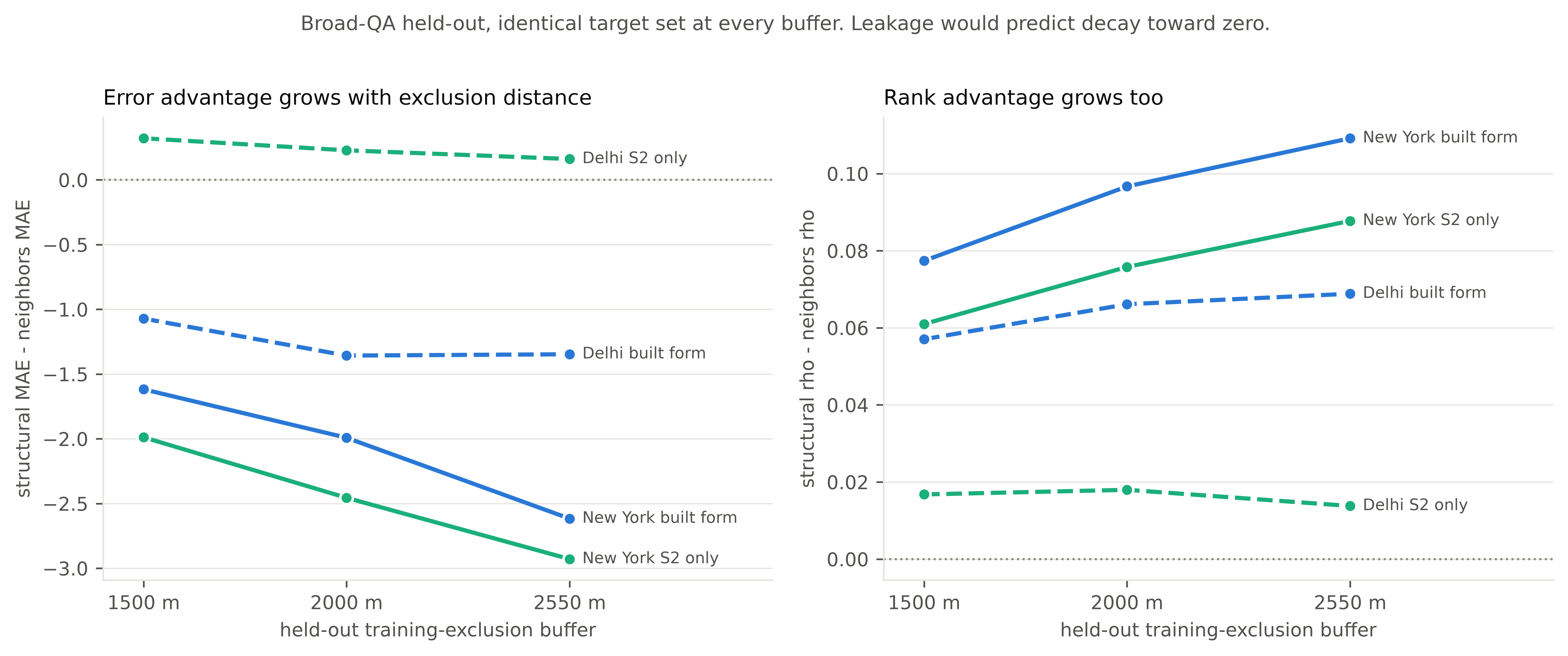
Every line moves away from zero as the buffer widens. Leakage predicts the opposite. New York built form goes −1.618 → −1.992 → −2.617 in MAE advantage and +0.077 → +0.097 → +0.109 in rank advantage.
This does not prove no leakage exists. It shows that whatever the structural prior is contributing survives, and strengthens, as local observations are withdrawn, which is the opposite of a leak.
8c. The substitution mechanism
Section 8b's growth has a direct reading. As the buffer widens, both methods degrade and the information available to either shrinks. The question is how fast.
"""Degradation of each method between the 1500 m and 2550 m buffers."""
def degradation(frame):
    o = frame[(frame.fold.astype(str) == "all") & (frame.radiance_decile.astype(str) == "all")]
    p = o.pivot_table(index=["city_id", "proxy", "method"], columns="buffer_m", values="mae")
    d = (p[2550.0] - p[1500.0]).rename("degradation").reset_index()
    return d

deg = degradation(hb)
rows = []
for city in CITIES:
    for proxy in ["built_form_primary", "s2_only_ablation"]:
        n = deg[(deg.city_id == city) & (deg.proxy == proxy) &
                (deg.method == "neighbors_only_prediction")].degradation.iloc[0]
        s = deg[(deg.city_id == city) & (deg.proxy == proxy) &
                (deg.method == "structural_prediction")].degradation.iloc[0]
        rows.append({"city": CITY_LABEL[city],
                     "proxy": "built form" if "built" in proxy else "S2 only",
                     "neighbors_only_degradation": round(n, 3),
                     "structural_degradation": round(s, 3),
                     "skill_retained_pct": round(100 * (1 - s / n), 1)})
display(pd.DataFrame(rows))
print("Skill retained = 1 - (structural degradation / neighbors degradation).")
print("Higher means the structural prior substitutes better for withdrawn observations.")
| city | proxy | neighbors_only_degradation | structural_degradation | skill_retained_pct | |
|---|---|---|---|---|---|
| 0 | New York | built form | 1.671 | 0.672 | 59.8 |
| 1 | New York | S2 only | 1.671 | 0.730 | 56.3 |
| 2 | Delhi | built form | 0.810 | 0.534 | 34.1 |
| 3 | Delhi | S2 only | 0.810 | 0.649 | 19.8 |
Skill retained = 1 - (structural degradation / neighbors degradation).
Higher means the structural prior substitutes better for withdrawn observations.
New York built form: neighbors-only degrades by +1.671 MAE between 1500 m and 2550 m; the structural prediction degrades by only +0.672. Roughly 60% of the skill lost by pure spatial interpolation is recovered by the structural prior.
This indicates how this method might be useful, even within cell (ie upsampling to higher resolution). In practice you are not predicting a held-out cell; you are allocating within a cell, where there is no local observation at the target scale at all. The withdrawn-observation limit is what matters, and structure holds up better there than interpolation does. The caveat here is scale...if density of structure scales differently (reasonable to think) at smaller resolutions, then be careful not to over-extend this.
Still, this seems to validate that knowing structure really helps us understand light radiance.
8d. The headline held-out result
Now that the mechanism and the leakage checks are established, the headline number is the expected consequence rather than the discovery.
"""Headline held-out table at the 2550 m primary buffer."""
prim = hb[(hb.buffer_m == 2550) & (hb.fold.astype(str) == "all") &
          (hb.radiance_decile.astype(str) == "all")]
wide = prim.pivot_table(index=["city_id", "proxy"], columns="method",
                        values=["mae", "rmse", "spearman"])

folds = hb[(hb.buffer_m == 2550) & (hb.fold.astype(str) != "all") &
           (hb.radiance_decile.astype(str) == "all")]
fp = folds.pivot_table(index=["city_id", "proxy", "fold"], columns="method", values="mae")
improved = ((fp["structural_prediction"] < fp["neighbors_only_prediction"])
            .groupby(level=[0, 1]).sum())

head = pd.DataFrame({
    "city": [CITY_LABEL[c] for c, _ in wide.index],
    "proxy": ["built form" if "built" in p else "S2 only" for _, p in wide.index],
    "neighbors MAE": wide[("mae", "neighbors_only_prediction")].values,
    "structural MAE": wide[("mae", "structural_prediction")].values,
    "neighbors RMSE": wide[("rmse", "neighbors_only_prediction")].values,
    "structural RMSE": wide[("rmse", "structural_prediction")].values,
    "structural rho": wide[("spearman", "structural_prediction")].values,
    "folds improved": [f"{improved.loc[i]}/5" for i in wide.index],
})
display(head.round(3))
| city | proxy | neighbors MAE | structural MAE | neighbors RMSE | structural RMSE | structural rho | folds improved | |
|---|---|---|---|---|---|---|---|---|
| 0 | Delhi | built form | 13.493 | 12.147 | 19.615 | 18.660 | 0.857 | 4/5 |
| 1 | Delhi | S2 only | 13.493 | 13.655 | 19.615 | 20.256 | 0.802 | 2/5 |
| 2 | New York | built form | 18.717 | 16.100 | 30.433 | 28.199 | 0.879 | 5/5 |
| 3 | New York | S2 only | 18.717 | 15.787 | 30.433 | 27.539 | 0.857 | 5/5 |
Built form improves MAE and RMSE in both cities and improves fold MAE in 5/5 New York folds and 4/5 Delhi folds. The single adverse Delhi fold worsens by 0.044 radiance units, which is noise at this scale. Delhi S2-only is worse overall and improves only 2/5 folds.
Strict-QA footnote: built form improved 5/5 folds in both cities under strict QA. The broad contract is marginally less favorable and is reported as primary anyway, because that's what I had on hand.
Two things this table does not say. It does not say the 10 m field is accurate: every number here is a coarse native-cell prediction. And New York S2-only beats built form (15.787 vs 16.100 MAE), which section 4 explains was recorded and deliberately not acted on.
8e. Water: an out-of-model check
Nothing above tests where within a cell the light goes. Water is the one place we have a weak prior that is genuinely outside the operator: open water should not emit much artificial light, and where VIIRS reports radiance over open water it is largely spill from the shore, atmospheric halo, and the sensor's own response width. Not light originating there. (boats being the important exception).
So: does structural allocation move radiance off open water relative to the direct upsample, and does it do so for structural reasons rather than by smoothing?
Metric basis (stated once, used throughout this section). Reduction fractions
are computed on common support with a positive-direct-radiance denominator,
from the broad-QA water_inland_ratio table for built form. The S2 ablation uses
the strict region_metrics table on the same basis, per section 0. Water is
defined by a separately acquired Overture 2026-06-17.0 areal-water reference,
not the JRC prior used inside the proxy, so the check is not circular.
"""Over-water allocation vs direct upsample. One metric basis, stated in section 8e."""
wb = pd.read_csv(ARTIFACTS["water_broad"])
ws = pd.read_csv(ARTIFACTS["water_strict"])

rows = []
for city in CITIES:
    r = wb[(wb.city_id == city) & (wb.region == "mapped_water")].iloc[0]
    i = wb[(wb.city_id == city) & (wb.region == "matched_inland_low_proxy")].iloc[0]
    rows.append({"city": CITY_LABEL[city], "proxy": "built form", "QA contract": "broad",
                 "water_reduction_pct": 100 * r.reduction_fraction_vs_direct,
                 "inland_control_reduction_pct": 100 * i.reduction_fraction_vs_direct})
    rs = ws[(ws.city_id == city) & (ws.proxy == "s2_only_ablation") &
            (ws.region == "mapped_water")].iloc[0]
    isx = ws[(ws.city_id == city) & (ws.proxy == "s2_only_ablation") &
             (ws.region == "matched_inland_low_proxy")].iloc[0]
    rows.append({"city": CITY_LABEL[city], "proxy": "S2 only", "QA contract": "strict",
                 "water_reduction_pct": 100 * rs.reduction_fraction_vs_direct,
                 "inland_control_reduction_pct": 100 * isx.reduction_fraction_vs_direct})

water = pd.DataFrame(rows)
water["water_minus_inland_pp"] = (water.water_reduction_pct
                                  - water.inland_control_reduction_pct)
display(water.round(1))
| city | proxy | QA contract | water_reduction_pct | inland_control_reduction_pct | water_minus_inland_pp | |
|---|---|---|---|---|---|---|
| 0 | New York | built form | broad | 39.6 | 81.0 | -41.4 |
| 1 | New York | S2 only | strict | 6.8 | 68.6 | -61.7 |
| 2 | Delhi | built form | broad | 52.6 | 55.0 | -2.4 |
| 3 | Delhi | S2 only | strict | -19.0 | 70.5 | -89.5 |
"""The uniform null: isolating structure from smoothing.

Shares are computed on the shoreline table's own basis (all valid pixels), which
is a DIFFERENT denominator from the reduction fractions above. Both the absolute
change and the share change are reported so the basis is never ambiguous.
"""
sl = pd.read_csv(ARTIFACTS["shoreline_summary"])
rows = []
for city in CITIES:
    d = sl[(sl.city_id == city) & (sl.configuration == "direct_upsample")].iloc[0]
    u = sl[(sl.city_id == city) &
           (sl.configuration == "uniform_normalized_convolution")].iloc[0]
    b = sl[(sl.city_id == city) &
           (sl.configuration ==
            "built_form_primary__no_water_prior__circular_mean_reference")].iloc[0]
    for name, r in [("uniform null", u), ("built form", b)]:
        rows.append({
            "city": CITY_LABEL[city], "method": name,
            "over_water_abs_change_pct":
                100 * (r.allocated_radiance_over_water
                       / d.allocated_radiance_over_water - 1),
            "over_water_share_change_pct":
                100 * (r.allocated_radiance_over_water_share
                       / d.allocated_radiance_over_water_share - 1),
        })
display(pd.DataFrame(rows).round(1))
print("Basis: shoreline summary.csv, all valid pixels. Strict contract "
      "(the full water factorial was\nnever re-run under broad). Not "
      "interchangeable with the reduction fractions in the previous cell.")
| city | method | over_water_abs_change_pct | over_water_share_change_pct | |
|---|---|---|---|---|
| 0 | New York | uniform null | 3.3 | 4.3 |
| 1 | New York | built form | -42.0 | -40.7 |
| 2 | Delhi | uniform null | 4.8 | 4.8 |
| 3 | Delhi | built form | -52.8 | -52.1 |
Basis: shoreline summary.csv, all valid pixels. Strict contract (the full water factorial was
never re-run under broad). Not interchangeable with the reduction fractions in the previous cell.
The uniform null is what would happen if we "just smoothed". Uniform normalized convolution, the same kernel, the same numerator, a flat proxy (i.e. no structure), increases over-water radiance (share +4.3% New York, +4.8% Delhi; absolute +3.3% and +4.8%). This is intuitive. Smoothing alone spreads shore light further out over the water. Built form moves it the other way, substantially. So the reduction is attributable to the structural prior, not to blurring.
This is a truly valuable find because it provides a method for making measures of radiance more precise in the very frequent case of urban areas that contain a lot of water.
The matched inland low-proxy control (areas of comparable structural emptiness that are not water, like parks), shows an even larger reduction: 81.0% versus 39.6% in New York. This indicates that this method is effective at constraining radiance where there are no light sources, independent of the type of surface areas (water or dark empty land).
"""Figure: water is not special. The inland low-proxy control reduces more."""
fig, ax = plt.subplots(figsize=(8.5, 3.8))
sub = water[water.proxy == "built form"]
xs = np.arange(len(sub))
w = 0.36
ax.bar(xs - w / 2, sub.water_reduction_pct, w * 0.92, color=BLUE,
       edgecolor="white", linewidth=1.2, label="mapped water (Overture reference)")
ax.bar(xs + w / 2, sub.inland_control_reduction_pct, w * 0.92, color=ORANGE,
       edgecolor="white", linewidth=1.2, label="matched inland low-proxy control")
for x, (_, r) in zip(xs, sub.iterrows()):
    ax.annotate(f"{r.water_reduction_pct:.1f}%", (x - w / 2, r.water_reduction_pct),
                ha="center", va="bottom", xytext=(0, 3), textcoords="offset points",
                fontsize=8, color=INK_2)
    ax.annotate(f"{r.inland_control_reduction_pct:.1f}%",
                (x + w / 2, r.inland_control_reduction_pct),
                ha="center", va="bottom", xytext=(0, 3), textcoords="offset points",
                fontsize=8, color=INK_2)
ax.set_xticks(xs); ax.set_xticklabels(sub.city)
ax.set_ylabel("reduction vs direct upsample (%)")
ax.set_title("Reduction over water is not larger than over comparable dry low-proxy land")
ax.legend(loc="upper right")
ax.grid(axis="y"); ax.set_axisbelow(True)
fig.tight_layout()
plt.savefig(SAVEFIG_PATH / "water-control.png", dpi=300, bbox_inches="tight")
plt.close(fig)
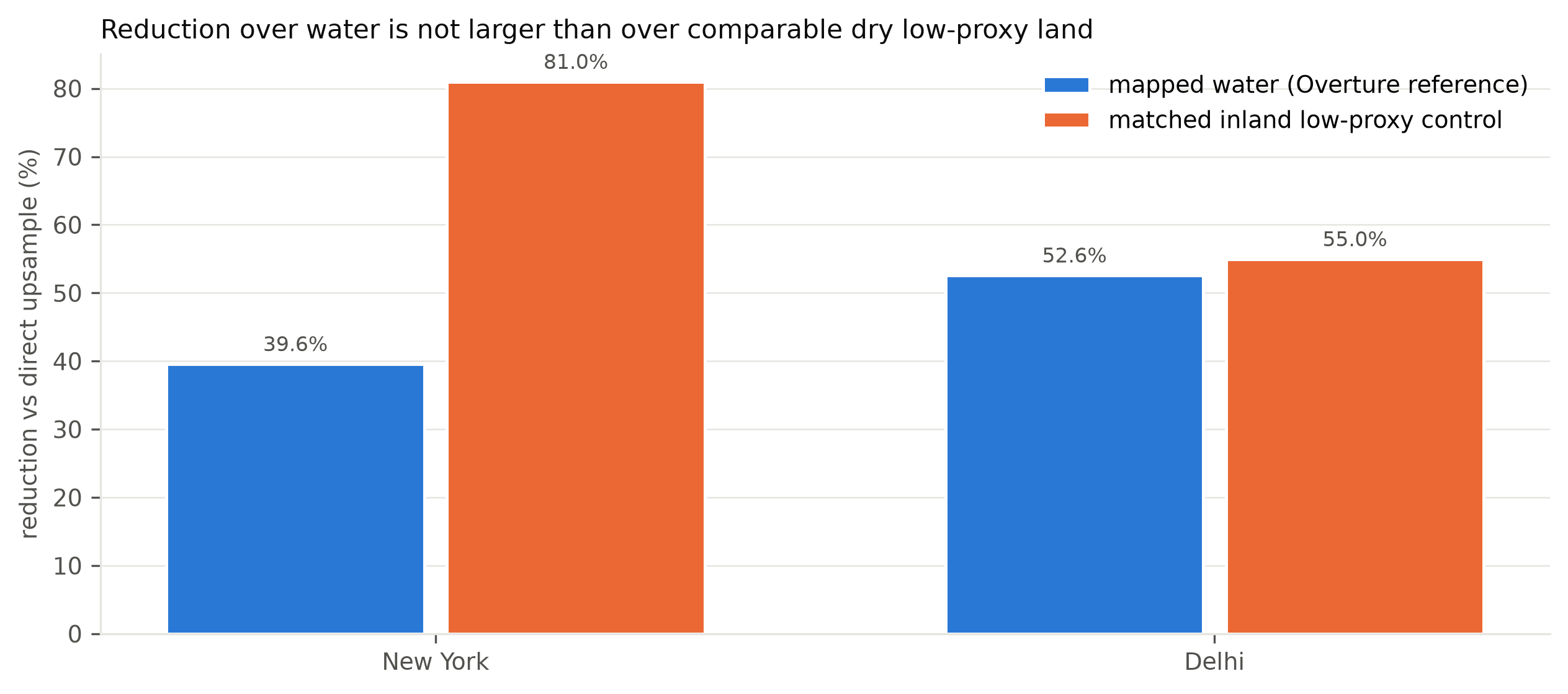
8f. Delhi S2-only: a worked failure
"""Four independent diagnostics for Delhi S2-only."""
g0 = pd.read_csv(ARTIFACTS["gate0_s2"])
delhi_g0 = g0[g0.get("city_id", g0.columns[0]).astype(str).str.contains("delhi", case=False)]

heldout_delhi = head[(head.city == "Delhi") & (head.proxy == "S2 only")].iloc[0]
gain_delhi = gp[(gp.city_id == "india_delhi") & (gp.proxy == "s2_only_ablation") &
                (gp.gain_stratum == ">=1.25")].iloc[0]
water_delhi = water[(water.city == "Delhi") & (water.proxy == "S2 only")].iloc[0]

evidence = pd.DataFrame([
    {"#": 1, "diagnostic": "Gate 0 shape (strict)",
     "value": "mound-shaped; passes all positive-correlation thresholds",
     "verdict": "missed by the rule"},
    {"#": 2, "diagnostic": "Held-out MAE, 2550 m (broad)",
     "value": f"{heldout_delhi['structural MAE']:.3f} vs "
              f"{heldout_delhi['neighbors MAE']:.3f} baseline "
              f"({heldout_delhi['folds improved']} folds)",
     "verdict": "worse than interpolation"},
    {"#": 3, "diagnostic": "Gain asymmetry, >=1.25 stratum (broad)",
     "value": f"{gain_delhi.structural_minus_neighbors_absolute_error:+.3f}",
     "verdict": "steepest of all four combinations"},
    {"#": 4, "diagnostic": "Over-water allocation vs direct (strict)",
     "value": f"{water_delhi.water_reduction_pct:+.1f}% reduction "
              f"(i.e. {-water_delhi.water_reduction_pct:+.1f}% MORE radiance on water)",
     "verdict": "wrong direction"},
])
display(evidence)
| # | diagnostic | value | verdict | |
|---|---|---|---|---|
| 0 | 1 | Gate 0 shape (strict) | mound-shaped; passes all positive-correlation ... | missed by the rule |
| 1 | 2 | Held-out MAE, 2550 m (broad) | 13.655 vs 13.493 baseline (2/5 folds) | worse than interpolation |
| 2 | 3 | Gain asymmetry, >=1.25 stratum (broad) | +3.407 | steepest of all four combinations |
| 3 | 4 | Over-water allocation vs direct (strict) | -19.0% reduction (i.e. +19.0% MORE radiance on... | wrong direction |
Pre-monsoon Delhi presents bare soil and an exposed Yamuna channel that are spectrally bright, low-NDVI, and non-water. This is the exact signature the S2-only proxy treats (incorrectly) as built-up. So the proxy places allocation weight on a dry riverbed and surrounding bare ground, which is why it adds radiance over mapped water (+19.0%) instead of removing it, why its upper-gain stratum is the most damaging of the four, and why it under-performs plain spatial interpolation.
New York's S2-only proxy does not fail this way because leaf-off New York has no comparable bare-bright surface, which is why it looks good there (section 8d) and is precisely why proxy selection on held-out performance would have been a trap.
The transferable lesson is not "don't use S2." It is: a spectral proxy encodes a
seasonal, regional surface hypothesis, and a screening gate built only on
correlation sign will not catch it. That is GATE0-MONOTONICITY-001, and it is
the finding I expect others to take note of.
8g. A couple notes
Here we ask whether disaggregation amplifies sensitivity to lunar irradiance, cloud state, snow, retrieval age, or quality flags relative to the baseline. It does not.
The operator has no mechanism for observation normalization: it does not model lunar phase, aerosol, or view angle, so any apparent improvement must be attributed to smoothing, and any reduction relative to direct (0.2479 → 0.1755) is smoothing by construction.
Kernel sensitivity identifies nothing about the true sensor response. Wider Gaussians produce worse reaggregation consistency (New York: 6.29 → 7.61 → 10.21 for 750/1000/1500 m FWHM) and less valid area (95.2% → 90.6% → 80.9%), because four-sigma truncation diminishes the analysis square's edges. Those two move together, so the comparison is confounded: you cannot tell whether the wider kernel is worse because it is a worse model of the PSF or because it is evaluated on a harder remnant.
9. Data and experiment contracts
The machine-readable version is the authority; it is printed verbatim below rather than paraphrased.
"""The final evidence classification, verbatim."""
ev = load_json(ARTIFACTS["evidence_v2"])

print("CLASSIFICATION:", ev["classification"].upper().replace("_", " "))
print("\n" + "=" * 78)
print("EXPERIMENT CONTRACT")
print("=" * 78)
for k, v in ev["experiment_contract"].items():
    print(f"\n{k}:\n  {v}")

print("\n" + "=" * 78)
print("SUPPORTED CLAIMS")
print("=" * 78)
for c in ev["supported_claims"]:
    print(f"  [+] {c}")

print("\n" + "=" * 78)
print("UNSUPPORTED CLAIMS -- language that may not be used")
print("=" * 78)
for c in ev["unsupported_claims"]:
    print(f"  [-] {c}")

print("\n" + "=" * 78)
print("MIXED FINDINGS")
print("=" * 78)
for c in ev["mixed_findings"]:
    print(f"  [~] {c}")

print("\n" + "=" * 78)
print("INHERITED EVIDENCE")
print("=" * 78)
for c in ev["inherited_evidence"]:
    print(f"  [<] {c}")
CLASSIFICATION: COVERAGE COMPLETE BOUNDED METHOD RESULT

==============================================================================
EXPERIMENT CONTRACT
==============================================================================

fine_grid_limit:
  the 10 m products are structurally allocated observation fields, not independently observed or calibrated 10 m radiance

objective:
  test whether a static fine-grid structural proxy can allocate coarse VNP46A2 radiance more plausibly than declared null allocations while VNP46A2 remains the radiometric authority

primary_estimand:
  native-cell broad-QA held-out prediction error under the frozen 2550 m PSF-support exclusion

==============================================================================
SUPPORTED CLAIMS
==============================================================================
  [+] all v2 primary and baseline COGs have complete two-city spatial support
  [+] the New York S2-only broad-QA sensitivity has zero radiance-neighborhood gaps; remaining invalid pixels are unchanged S2 proxy-support gaps
  [+] on the frozen native-cell cohort, broad-QA built form improves overall MAE and RMSE in both cities at the 2550 m buffer
  [+] the radiance-blind gain asymmetry persists under broad QA in all four city-by-proxy comparisons
  [+] the broad water-versus-inland result remains consistent with general low-proxy reallocation rather than a water-specific effect

==============================================================================
UNSUPPORTED CLAIMS -- language that may not be used
==============================================================================
  [-] observed or calibrated 10 m nighttime radiance
  [-] pixel-level accuracy from gain strata
  [-] equivalent quality of MQF 0 and MQF 1
  [-] broad-QA daily observation-condition correction
  [-] validated water correction or recovered physical emissions

==============================================================================
MIXED FINDINGS
==============================================================================
  [~] Delhi built form improves broad-QA MAE in 4 of 5 folds; fold 3 worsens by only 0.044 radiance units
  [~] New York S2-only remains lower-error than built form, while Delhi S2-only remains negative overall
  [~] broad QA removes support holes but admits MQF 1 and lower cloud-mask quality
  [~] only the New York S2-only spatial raster was regenerated under broad QA; the Delhi S2-only spatial sensitivity remains strict-v1 and is not a like-for-like cross-city map comparison

==============================================================================
INHERITED EVIDENCE
==============================================================================
  [<] the daily observation-condition propagation audit remains strict-QA conservative sensitivity evidence and is not relabeled as broad-QA validation
The scope/limits of this experiment
Validated: coarse-cell prediction. The structural prior predicts held-out native-cell radiance better than spatial interpolation, in both cities, at the physics-derived exclusion distance, with an advantage that grows as local observations are withdrawn. That is a real, reproducible, leakage-checked result.
Not validated: the within-cell allocation. Nothing here observes light at 10 m. The one out-of-model directional check (water) survives as general low-proxy reallocation, attributable to structure rather than smoothing, but not as a water-specific or magnitude-accurate correction.
The gap between those two is not rhetorical, and it is not closable with more of the same data. It needs an independent fine-grid nighttime observation (e.g. SGDSAT or ISS), which is section 10.
A useful way to hold it: the operator is a defensible re-expression of a coarse observation onto a structural basis, which contains an explicit error structure. It is not a measurement of 10 m nighttime radiance, and the products must never be described as one.
10. Future work
Ordered by rough effort/benefit.
1. Edge-spread estimation from long straight shorelines. The highest-value follow-on available in data already built. The shoreline-distance bands and infrastructure strata from section 8e can be replicated: along a long, straight, high-contrast land/water boundary, the observed cross-shore radiance profile is an edge-spread function, and its derivative estimates a line spread function. This would replace the declared circular kernel with something partially measured, with no new acquisitions. It will not give the full 2-D PSF, and scan-angle dependence remains unidentified, but it gives a bounded estimate.
2. SDGSAT-1 as an independent fine-grid reference. This is the best way to validate the sub-500m resolution. But it requires acquisition time, calibration status, cloud cover, georegistration method and uncertainty, and license before any comparison is made, and it must be treated as an independent reference with stated limits, not as ground truth.
3. Remove-before-fine-grid-convolution. The stronger held-out test: remove held-out radiance before reprojection and convolution, produce the full allocation, and reaggregate to exact native polygons. The completed run is a coarse structural-gain analogue; this would be the operator-level test. It is expensive because every fold requires a full fine-grid rerun.
4. Historical OSM vintage sensitivity. Contemporary Overture allocates 2024 radiance, which as noted is a temporal mismatch. Completing it would address this concern, but OSM-only versus multi-source Overture means it is a combined source-coverage and vintage sensitivity, never a clean temporal experiment.
5. Residual autocorrelation and structure attribution. Signed residuals look broadly balanced at city scale with no obvious gradient or seam, which is not evidence of spatial independence. Local conditioning by roads, waterways, development edges, and radiance decile remains plausible and untested.
6. The causal application. The Debnath et al. heatwave-response benchmark is the natural first real use: does a measurement layer with an explicit error structure change the estimated effect, and does the trust-indicator stratum predict where it changes most?
11. Data provenance, licensing, and reproduction
Provenance
| Input | Source | Version / pin | Notes |
|---|---|---|---|
| Nighttime radiance | NASA Black Marble VNP46A2 (DNB_BRDF_Corrected_NTL + QA bands) |
2024-01-11 to 2024-04-20 | NASA-led mission data are CC0 unless marked otherwise; cite VNP46A2.002. Accessed via Earth Engine. Collection 2. The Oct 2024 NASA C2 guide and the EE catalog disagree about MQF 1, which is why both QA contracts are retained |
| Daytime structure | Sentinel-2 SR Harmonized + Cloud Score+ | same window | Copernicus Sentinel free/full/open terms; modified outputs require the Copernicus source notice. Cloud Score+ is CC BY 4.0. B11/B12 and derived indices retain 20 m effective resolution though sampled at 10 m |
| Buildings and roads | Overture Maps | 2026-07-22.0 |
Buildings and Transportation themes are ODbL and require Overture/OSM attribution plus applicable upstream notices. A contemporary proxy used to allocate 2024 radiance |
| Water reference (validation) | Overture areal water | 2026-06-17.0 |
Base theme is ODbL. Deliberately separate from the proxy's internal prior. Primarily OSM-derived; line-only waterways unbuffered, pools/wastewater excluded |
| Persistent-water prior (internal) | JRC Global Surface Water occurrence | 1984–2021, 30 m | A temporal frequency, not a 10 m spatial fraction and not a 2024 observation. Inactive in the reporting primary (no_water_prior) |
Two provenance caveats that affect interpretation rather than mechanics. The structural layers are contemporary, not 2024: Overture building coverage is uneven across cities and improves over time, so New York and Delhi are not equally well mapped, and neither is mapped as of the radiance window. And the water reference, while independent of the JRC prior, is not independent of OpenStreetMap, which also underlies the road and building layers; a shoreline mis-mapped in OSM is mis-mapped in both.
Reproduction
The software in the standalone repository is licensed under the BSD 3-Clause
License. Source use and derived-artifact redistribution remain subject to
upstream terms. The complete retrieval, redistribution, and figure-attribution
record is in docs/data-licenses.md.
Attribution for the maps and figures in this notebook. Nighttime radiance contains modified NASA VIIRS VNP46A2 Collection 2 data (2024), DOI: 10.5067/VIIRS/VNP46A2.002, accessed through Google Earth Engine. Contains modified Copernicus Sentinel data 2024. Cloud-quality data: Google Earth Engine Cloud Score+, CC BY 4.0. Map and structural data: © OpenStreetMap contributors, Overture Maps Foundation; ODbL 1.0. Persistent-water data, where shown: Source: EC JRC/Google.
What reruns offline: the operator, all Gate 1 invariants, held-out folds,
shoreline and water analyses, sensitivity tables, and every figure in this
notebook — all from the local artifact tree. Compact evidence is versioned under
artifacts/; users generate and store the full-size COGs locally. They are not
committed to GitHub or distributed through a project-hosted raster archive.
What does not: anything that touches Earth Engine (Gate 0 sampling, the S2
composite, VNP median construction, the daily stack). Those need a registered
GCP project with the EE API enabled. Set NTL_PSF_EE_PROJECT and
NTL_PSF_EE_DRIVE_FOLDER in the local shell; their values are deliberately
absent from configs/psf_disaggregation.yaml. The
raw exports land in Google Drive and are validated on download against the
recorded CRS, 5200x5200 shape, transform, band order, and COG layout before any
operator run is permitted.
"""Reproduction check against the private-runtime frozen configuration."""
FROZEN_CONFIG_SHA256 = "9a0338232881f7d6353259672d6a3c45f83b50d67dacbc00f3d8d986b72d718a"
config_bytes = CONFIG_PATH.read_bytes()
print(f"public redacted config sha256: {hashlib.sha256(config_bytes).hexdigest()}")
print(f"frozen runtime config sha256: {FROZEN_CONFIG_SHA256}")

manifests = {
    "full-city broad (v2)": BROAD / "artifact_manifest.json",
    "full-city strict (v1)": STRICT / "artifact_manifest.json",
    "held-out broad (v3)": VAL / "gate2/heldout/v3_physics_buffered_native_cell_broad_qa/manifest.json",
    "shoreline (v1)": VAL / "gate2/shoreline/v1_overture_mapped_water/manifest.json",
    "sensitivity (v1)": VAL / "gate2/sensitivity/v1_full_city_sensitivity/manifest.json",
    "observation conditions (v1)": VAL / "gate2/observation_conditions/v1_daily_coarse_operator/manifest.json",
}
rows = []
for name, path in manifests.items():
    if not path.exists():
        rows.append({"manifest": name, "configuration_sha256": "MISSING"}); continue
    blob = json.dumps(load_json(path))
    import re
    hits = sorted(set(re.findall(r"\b[0-9a-f]{64}\b", blob)))
    cfg = [h for h in hits if h == FROZEN_CONFIG_SHA256]
    rows.append({"manifest": name,
                 "configuration_sha256": (cfg[0][:16] + "...") if cfg else "not found"})
display(pd.DataFrame(rows))
public redacted config sha256: 67b984311cda71bd275afaff47ad517649e857e9bd1b5959d664945b3e7a1796
frozen runtime config sha256: 9a0338232881f7d6353259672d6a3c45f83b50d67dacbc00f3d8d986b72d718a
| manifest | configuration_sha256 | |
|---|---|---|
| 0 | full-city broad (v2) | 9a0338232881f7d6... |
| 1 | full-city strict (v1) | 9a0338232881f7d6... |
| 2 | held-out broad (v3) | 9a0338232881f7d6... |
| 3 | shoreline (v1) | 9a0338232881f7d6... |
| 4 | sensitivity (v1) | 9a0338232881f7d6... |
| 5 | observation conditions (v1) | 9a0338232881f7d6... |